Cochran-Armitage Trend Test: Hypotheses, Assumptions, and Application

1. The Specific Scenario for the Cochran-Armitage Test

The Cochran-Armitage test is not a general-purpose tool; it's designed for a very specific, yet common, situation in data analysis: a contingency table where one variable is binary (two categories) and the other is ordinal (k ordered categories). This results in a 2×k or k×2 table.

Typical scenarios include:

• Dose-Response Studies: Testing if the proportion of patients recovering (binary: recovered/not recovered) increases across different drug dosage levels (ordinal: low, medium, high).
• Epidemiology: Examining if the prevalence of a disease (binary: present/absent) shows a trend across ordered age groups (ordinal: 20-29, 30-39, 40-49).
• Surveys: Assessing if the proportion of respondents who agree with a statement (binary: agree/disagree) changes across education levels (ordinal: high school, bachelor's, master's).

This table neatly summarizes when to use the Cochran-Armitage test compared to other trend tests you might encounter.

To get a clearer picture of this setup, the following reading introduces the C-A test and presents a clear example.

2. Hypotheses and the Scoring Mechanism

As you've just read, the C-A test goes beyond the simple "association vs. no association" question. Its hypotheses are specifically about a trend.

• Null Hypothesis ($H_0$): There is no trend in the proportions of the binary outcome across the ordered categories. In other words, the proportion is the same for all levels of the ordinal variable.
• Alternative Hypothesis ($H_A$): There is a linear trend (either increasing or decreasing) in the proportions across the ordered categories.

To test this, the C-A test assigns numerical scores to the ordinal categories. For example, 'Low Dose' = 1, 'Medium Dose' = 2, 'High Dose' = 3. It then essentially tests whether the correlation between the binary outcome (coded as 0 and 1) and these scores is significantly different from zero.

The resulting test statistic, often denoted as $M^2$ or $Z^2$, is compared to a chi-square distribution with 1 degree of freedom.

The Crucial Choice of Scores

The scores you assign matter. While the test is often robust to different scoring systems, it's an important assumption.

• Equally Spaced Scores (e.g., 1, 2, 3, 4): This is the most common and default approach. It assumes the "distance" between each category is equal. This is a reasonable starting point if you have no other information.
• Mid-ranks: This is a non-parametric approach that can be useful if the categories have very different numbers of observations.
• Substantive Scores: If your categories represent something with a natural numerical value (e.g., the midpoint of age ranges like 25, 35, 45), using those values as scores is often the best choice.

The next reading dives deeper into this concept and also explains the power advantage of this approach.

As the reading suggests, if you are uncertain about scores, a good practice is a sensitivity analysis: try a few different reasonable scoring systems and see if your conclusion changes.

3. Application and Interpretation

Let's see how this works in practice. The Cochran-Armitage test statistic is actually a component of the overall Pearson chi-square statistic. It partitions the total variation into two parts:

1. Variation due to a linear trend (1 df).
2. Variation due to departures from a linear trend ($k-2$ df).

Total Chi-Square ($k-1$ df) = Trend Chi-Square (1 df) + Departure from Linearity Chi-Square ($k-2$ df)

When we perform a C-A test, we are focusing only on that first component.

The image below shows a perfect example of this. We have a 2x5 table (binary outcome vs. 5-level ordinal predictor).

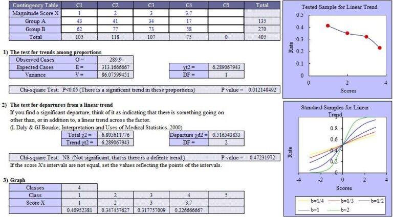
How to interpret the results:

1. Examine the Trend Test: Look at the p-value for the Cochran-Armitage test statistic (the one with 1 df).

   • If p < 0.05 (or your chosen alpha level), you reject the null hypothesis and conclude there is a statistically significant linear trend.
   • If p ≥ 0.05, you do not have sufficient evidence to claim a linear trend exists.

2. Determine the Direction of the Trend: The test statistic itself doesn't tell you if the trend is positive or negative. You must look at the data.

   • Calculate the proportions of the "success" category for each level of the ordinal variable.
   • Plot these proportions (as in the graph above) or simply observe if they consistently increase or decrease across the categories.

4. Assumptions

To use the Cochran-Armitage test correctly, you need to be aware of its assumptions:

1. Data Structure: The data is in a 2×k (or k×2) contingency table.
2. Variable Types: One variable is binary, and the other is ordinal.
3. Independence: The observations are independent.
4. Linearity: The test is specifically designed to detect a linear trend in proportions across the scored categories. It will have low power to detect complex, non-monotonic trends (like a U-shape), which we discussed in the previous lesson.
5. Sample Size: A common rule of thumb, mentioned in the resource LINK, is that the test is reliable when $n\bar{p}\bar{q}>5$, where $n$ is the total sample size, $\bar{p}$ is the overall proportion of successes, and $\bar{q}=1-\bar{p}$.

Conclusion

In this lesson, you've learned the specifics of the Cochran-Armitage trend test, a powerful tool for a common analytical scenario. You've moved beyond the general concept of trend tests to the practical details of one of its most important implementations.

Key Takeaways:

• Application: The C-A test is used for 2×k contingency tables to test for a trend in proportions across an ordinal variable for a binary outcome.
• Hypotheses: It tests the null of no trend against the alternative of a linear trend.
• Mechanism: It works by assigning numerical scores to the ordinal categories and testing for a correlation. The choice of scores is an important consideration.
• Power: The test statistic has 1 degree of freedom, making it more powerful for detecting linear trends than the general Pearson chi-square test.
• Interpretation: A significant result indicates a monotonic trend. You must inspect the proportions in the data to determine the trend's direction (increasing or decreasing).

Preview of the Next Lesson:

The Cochran-Armitage test is perfect for the ordinal-by-nominal case. But what if both of your variables are ordinal? For instance, what if you want to see if there's a trend between 'level of agreement' (e.g., strongly disagree to strongly agree) and 'income bracket' (e.g., low to high)? In our next lesson, we will cover the linear-by-linear association test, which extends these concepts to handle ordinal-by-ordinal tables.