Cochran-Armitage and Linear-by-Linear Association Tests

1. Applying the Cochran-Armitage Trend Test

Let's start with a classic scenario for the C-A test: a dose-response study. Imagine a clinical trial where patients are given different doses of a new drug, and we record whether they experience dizziness as a side effect.

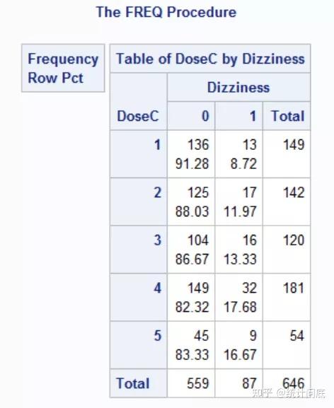
Why is the Cochran-Armitage test the right choice here?
Because we have one ordinal variable (DoseC) and one binary variable (Dizziness). We are not just interested in whether there's an association; we specifically want to know if the proportion of people experiencing dizziness shows a consistent trend (up or down) as the dose increases. A standard chi-square test would miss this nuance.

Interpreting the Output

Let's look at how to run and interpret this test using a similar example from a practical R guide. The example below involves one nominal variable ('Travel') and one ordinal variable ('Breakfast'). The principle is identical to our dose-dizziness case.

Let's break down the interpretation process, applying it to our dizziness example:

1. State the Hypotheses:

   • Null Hypothesis ($H_0$): The proportion of patients experiencing dizziness is the same across all dose levels (i.e., there is no trend).
   • Alternative Hypothesis ($H_A$): There is a linear trend in the proportion of patients experiencing dizziness as the dose level changes.

2. Examine the Test Result: The output from the test would give us a chi-square statistic and a p-value. In the breakfast example, the result was chi-squared = 8.6739, df = 2, p-value = 0.01308. If we ran this on our dizziness data, we would almost certainly get a very small p-value (p < .05). This tells us to reject the null hypothesis. There is statistically significant evidence of a trend.

3. Determine the Direction of the Trend: The p-value confirms a trend exists, but it doesn't tell us if it's positive or negative. For that, we simply inspect the contingency table. Look at the "Row Pct" for Dizziness=1 in the image above:

   • Dose 1: 8.72% experienced dizziness.
   • Dose 2: 12.00%
   • Dose 3: 20.00%
   • Dose 4: 31.08%
   • Dose 5: 35.82%
     The proportion clearly increases as the dose increases. Therefore, we conclude there is a significant positive trend.

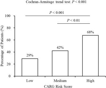
This type of result is often visualized in research papers with a simple bar chart, like the one below, which makes the trend immediately obvious.

2. Applying the Linear-by-Linear Association Test

Now, let's switch to a scenario where both variables are ordinal. We'll revisit the example of farm size and adoption of a new practice.

• Variable 1 (Rows): Farm Size ('Hobbyist', 'Mom-and-pop', 'Small', 'Medium', 'Large') - Ordinal
• Variable 2 (Columns): Adoption Level ('Always', 'Sometimes', 'Never') - Ordinal

Here, the C-A test is inappropriate because neither variable is binary. We need the linear-by-linear (LBL) association test to see if there's a monotonic relationship between farm size and adoption.

Let's walk through the interpretation steps for the LBL test:

1. State the Hypotheses:

   • Null Hypothesis ($H_0$): There is no linear association between farm size and adoption level.
   • Alternative Hypothesis ($H_A$): There is a linear association between farm size and adoption level.

2. Examine the Test Result: The reading showed a p-value of 0.0008761. Since this is much less than 0.05, we reject the null hypothesis. There is a significant linear association.

3. Determine the Direction of the Association: The test statistic itself (M^2 or Chisq) is always positive. To find the direction, you can:

   • Inspect the table: Look at the counts. 'Hobbyist' farms are concentrated in the 'Never' column (5 of 6). 'Large' farms are concentrated in the 'Always' column (2 of 2). This shows that as farm size increases, adoption tends to move towards 'Always'. This is a positive association.
   • Look at the Z-score (if available): The lbl_test output gives Z = -3.3276. A negative Z-score indicates a negative correlation. This might seem contradictory, but it depends on the numerical scores assigned to the categories. In R, factors are often scored based on their level order. If 'Adopt' is ordered c("Always", "Sometimes", "Never"), then 'Always' gets score 1, 'Sometimes' gets 2, and 'Never' gets 3. As farm size increases (higher score), the adoption level moves towards 'Always' (lower score). A higher score on one variable corresponds to a lower score on the other, which is a negative correlation. The interpretation is the same: larger farms are more likely to adopt the practice.

3. A Critical Limitation: Non-Linear Trends

It's vital to remember what these tests are for: detecting linear (or monotonic) trends. They gain their power by focusing on this specific type of association. The trade-off is that they can completely miss associations that are not linear.

Consider the example from the previous lesson's resource on the effect of a drug, where the success rate is low at low doses, high at medium doses, and low again at high doses. This is a "U-shaped" or non-monotonic association.

• A Pearson chi-square test would likely detect this association because it just checks if the proportions are different, regardless of pattern.
• A Cochran-Armitage or LBL test would likely find no significant trend because the initial increase is cancelled out by the later decrease. The overall linear correlation would be close to zero.

This is a key part of your functional understanding: if you have reason to suspect a non-linear association, a general chi-square test may be more appropriate.

Conclusion

You have now moved from the theory of trend tests to their practical application. You can now identify the correct test for your data and interpret the results to draw meaningful conclusions.

Key Takeaways:

• Cochran-Armitage Test: Use for ordinal-by-binary tables to test for a trend in proportions.
• Linear-by-Linear Association Test: Use for ordinal-by-ordinal tables to test for a linear association.
• Power: Both tests are generally more powerful than the standard Pearson chi-square test for detecting monotonic trends because they focus the analysis on a single degree of freedom.
• Interpretation is a Two-Step Process:
  1. Check the p-value to determine if a significant trend/association exists.
  2. Inspect the contingency table (e.g., row/column percentages) to determine the direction of the relationship.
• Limitation: These tests are designed for linear trends and will have low power to detect other patterns of association (e.g., U-shaped).

Preview of the Next Lesson:

So far, all the tests we've covered assume that the observations are independent. For example, in our tables, one person's response does not influence another's. But what if our data is paired or matched? For example, what if we measure a patient's opinion before and after a treatment? The standard chi-square test is invalid in this case. In the next lesson, we will begin exploring methods for analyzing such dependent data, starting with the McNemar test.