Understanding Confounding Variables

1. What is Confounding? A First Look

At its heart, confounding occurs when the effect of an exposure on an outcome is mixed up with the effect of a third, extraneous variable. This third variable is called a confounder.

Let's start with a video that provides an excellent and intuitive introduction to this concept using a couple of clear examples.

As the video explained, if we only look at ice cream sales and sunburn rates, we'd find a strong positive association. But it's absurd to think that eating ice cream causes sunburn. The real driver is the confounder, sun exposure, which influences both how much ice cream people buy and their risk of sunburn.

This relationship can be visualized with a causal diagram.

Formally, confounding is the distortion of the association between an exposure and an outcome by an extraneous third variable. This distortion can lead us to overestimate, underestimate, or even completely reverse the true association.

2. The Three Criteria for a Confounder

For a variable to be a confounder in a study, it must satisfy three specific conditions. Your ability to check for these criteria is a core part of the "functional understanding" you seek.

A variable is a confounder if:

1. It is a risk factor for the outcome (independent of the exposure).
2. It is associated with the exposure.
3. It is not on the causal pathway between the exposure and the outcome.

Let's explore these criteria using a more rigorous example.

Let's summarize the example from the reading:

• Exposure: Diabetes
• Outcome: Coronary Heart Disease (CHD)
• Potential Confounder: Hypertension

Here is how the three criteria were checked:

1. Associated with Outcome? Yes. Among non-diabetics, those with hypertension had a higher prevalence of CHD (5.5%) than those without (3.1%).
2. Associated with Exposure? Yes. People with hypertension were more likely to have diabetes (15.8%) than those without hypertension (4.9%).
3. Not on Causal Pathway? Yes. Based on biological knowledge, hypertension is not an intermediate step through which diabetes causes CHD. Both can independently contribute to heart disease.

Since hypertension met all three criteria, it is a confounder in the relationship between diabetes and CHD. The initial, crude analysis was therefore biased.

3. How Confounding Distorts Association: Simpson's Paradox

The most dramatic illustration of confounding is Simpson's Paradox, a phenomenon where a trend that appears in different groups of data disappears or reverses when these groups are combined. This is exactly what confounding does: it creates a misleading overall trend by hiding the real trend within subgroups.

The following video from TED-Ed provides a fantastic, clear explanation of this paradox.

Let's break down the hospital example from the video:

• Crude Association: Hospital A (900/1000 = 90% survival) looks better than Hospital B (800/1000 = 80% survival).
• Confounder: The initial health of the patients (good vs. poor).
• Stratified Association:
  • For patients in poor health, Hospital B was better (210/400 = 52.5% survival vs. 30/100 = 30% for Hospital A).
  • For patients in good health, Hospital B was also better (580/600 = ~97% survival vs. 870/900 = ~97% for Hospital A, but the video notes B is slightly better at >98%).

The overall result was distorted because Hospital B, being a better hospital, likely attracted more high-risk patients. This dragged down its overall survival rate, making it look worse in the crude analysis.

This reveals a key mathematical property of confounding:

When you have a confounder, the crude (overall) measure of association will be outside the range of the stratum-specific measures of association.

In the hospital example, the overall result (A > B) was different from the result in every single stratum (B > A).

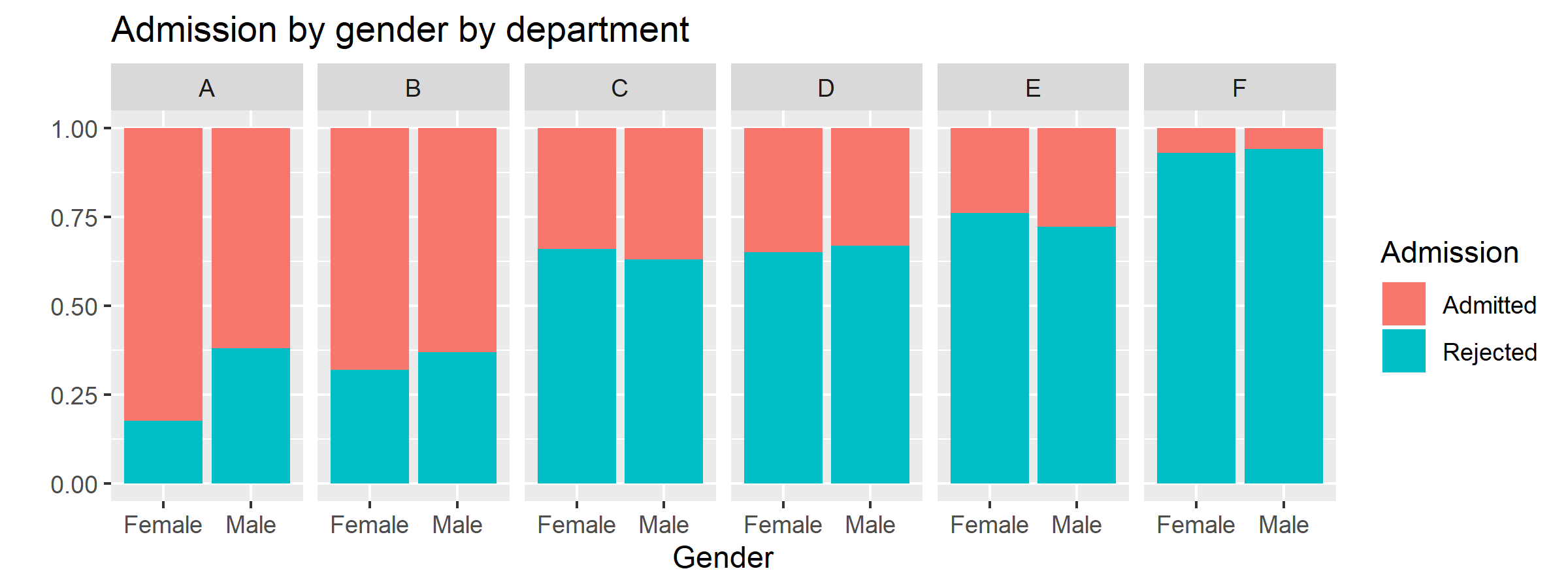
A famous real-world example of Simpson's Paradox occurred in the 1970s at UC Berkeley, where graduate school admissions data initially suggested a bias against female applicants.

To see the numerical effect of distortion, let's look at one final resource.

In this example, the crude risk ratio (1.13) suggested a very weak association between a high-fat diet and colon cancer. However, this was a distortion. The true association was stronger, as seen in the stratified risk ratios (1.29 and 1.68). The crude estimate was biased towards the null (a risk ratio of 1.0) because of confounding by vitamin use.

Conclusion

In this lesson, you've learned to identify one of the most significant threats to the validity of a statistical analysis: confounding. Ignoring it is not a minor oversight; it can lead you to draw conclusions that are the opposite of the truth.

Key Takeaways:

• Confounding is the distortion of an association between an exposure and an outcome by a third variable, the confounder.
• A variable is a confounder if it is associated with the outcome, associated with the exposure, and not on the causal pathway.
• Confounding can create a spurious association where none exists, or it can hide, diminish, or even reverse a real one.
• Simpson's Paradox is a classic example of confounding where the trend observed in aggregate data is the reverse of the trend observed within all subgroups.
• Identifying potential confounders requires both data analysis (checking the first two criteria) and subject-matter knowledge (checking the third criterion).

Preview of the Next Lesson:

Now that we can define confounding and understand the havoc it can wreak, the natural next question is: "What do we do about it?" In the next lesson, we will explore stratification as a fundamental technique to both identify the presence of confounding and to obtain an unbiased, adjusted measure of association. This will lead us directly to the Cochran-Mantel-Haenszel (CMH) test, a powerful tool for analyzing stratified tables.