Identifying Confounding in Contingency Tables with Stratification

1. The Logic of Stratification: Marginal vs. Partial Tables

The core idea of stratification is simple: if we suspect a variable is confounding our analysis, we can temporarily remove its influence by looking at the data within specific levels, or strata, of that variable. For example, if we think age is a confounder in a study of a new drug, we would analyze the data separately for "young patients," "middle-aged patients," and "old patients."

This process introduces some important terminology for the tables we create. A brief reading from a practical guide to the Cochran-Mantel-Haenszel test will help us define these terms.

To summarize the key ideas from that reading:

• The marginal table gives us the crude measure of association. This is the overall relationship we observe before accounting for any potential confounders.
• The partial tables give us stratum-specific measures of association. Each one shows the relationship within a single, more homogeneous subgroup.
• If a variable is a confounder, the crude odds ratio from the marginal table will be a distorted summary of the true association, which is better represented by the conditional odds ratios from the partial tables.

2. The Process: How to Identify Confounding

Now that we have the right terminology, how do we use these tables to formally identify confounding? The process is a direct comparison.

Let's watch a short video that illustrates this with a clear example. In the previous lesson, we saw examples where confounding created a spurious association. Here, we'll see stratification used to reveal that the initial association was indeed false.

The video demonstrates the most extreme case of confounding: an association that is entirely explained away. In practice, the effect is often more subtle. The general process for identification is summarized in the diagram below.

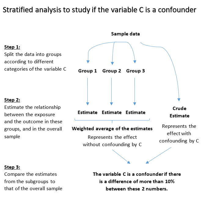
So, the key question is: how different do the crude and adjusted measures have to be?

While there is no universal cutoff, a common rule of thumb in epidemiology is that confounding is present if the crude and adjusted estimates differ by more than 10-20%.

The flowchart below illustrates this decision process. The "adjusted" measure (like ${\text{OR}}_{\text{MH}}$ for the Mantel-Haenszel odds ratio, which we'll cover soon) is a summary of the stratum-specific odds ratios.

The percentage change is typically calculated as:

3. A Detailed Numerical Example

Let's walk through a complete example to see this process in action with real numbers. The following video analyzes data from a cohort study to see if age confounds the relationship between sex and mortality.

This video will also introduce the Mantel-Haenszel adjusted rate ratio, which is a weighted average of the stratum-specific rate ratios. Think of it as the "summary" measure of association after controlling for the confounder.

Let's recap the findings from the video:

• Crude Rate Ratio: 1.1
• Adjusted Rate Ratio: 1.5

The crude analysis suggested a very small (10%) increase in mortality risk for men. However, after adjusting for age, the analysis showed a much larger (50%) increase in risk. The crude measure was heavily biased towards the null value of 1.0.

Using our rule of thumb:

Since 26.7% is well above the 15-20% threshold, we have strong evidence of confounding. The crude measure is misleading, and the adjusted measure should be reported.

4. When Stratification Fails

You rightly pointed out that knowing the limitations of a method is crucial. Stratification is intuitive and powerful, but it has a significant practical weakness.

The same video you just watched concludes with a discussion of this very point.

The key limitation is data sparsity.

• To control for one binary confounder, you create two strata.
• To control for two binary confounders, you need $2\times 2=4$ strata.
• To control for three, you need 8 strata, and so on.

As you create more and more strata, you spread your data thinner and thinner. Eventually, the number of individuals in each stratum becomes so small that you can no longer get reliable estimates of the odds ratio or rate ratio within those strata.

This is the primary reason why, in practice, multivariable regression models (like the logistic and Poisson regression models we will study later) are often preferred. They can mathematically adjust for many confounders simultaneously without needing to physically split the data into dozens of tiny subgroups.

Conclusion

In this lesson, we put the theory of confounding into practice. We learned how to use stratification not just as a conceptual tool, but as a direct analytical method to detect the presence of confounding in a dataset.

Key Takeaways:

• Stratification is the process of splitting data into subgroups (strata) based on the levels of a potential confounding variable.
• We can identify confounding by comparing the crude measure of association (calculated from the overall, or marginal, table) with an adjusted measure of association (a weighted average of the stratum-specific measures).
• A substantial difference between the crude and adjusted measures (e.g., >10-20%) is evidence of confounding, indicating the crude measure is biased.
• The main limitation of stratification is data sparsity: it becomes impractical when you need to control for several confounders at once, as the strata become too small.

Preview of the Next Lesson:

We have now seen how to use stratification to identify confounding by comparing crude and adjusted measures. The next logical step is to formalize this process. In the next lesson, we will learn about the Cochran-Mantel-Haenszel (CMH) test. This test allows us to formally test the null hypothesis of no association between an exposure and an outcome after controlling for a confounder across multiple strata. We will also look more closely at how the Mantel-Haenszel summary odds ratio is calculated and interpreted.