Subqueries and CTEs for Complex Queries

1. Understanding Subqueries

A subquery, also known as an inner query or nested query, is a SELECT statement that is nested inside another SQL statement. The result of the subquery is then used by the outer query. Let's break down the different types.

Non-Correlated Subqueries

A non-correlated subquery is an independent query whose result is calculated once and then passed to the outer query. It can be run on its own without any dependency on the outer query.

Let's watch a video that explains the two main types of non-correlated subqueries: scalar and multi-row.

To summarize the video's key points:

• Scalar Subquery: Returns a single value. Often used with comparison operators (=, >, <) in a WHERE clause.

  -- Find products with a price higher than the average price
  SELECT product_name, price
  FROM products
  WHERE price > (SELECT AVG(price) FROM products);
  

• Multi-Row Subquery: Returns a list of values in a single column. Often used with the IN or NOT IN operators.

  -- Find all customers who live in a country that has a 'Z' in its name
  SELECT first_name, last_name
  FROM customers
  WHERE country IN (SELECT country FROM countries WHERE country LIKE '%Z%');
  

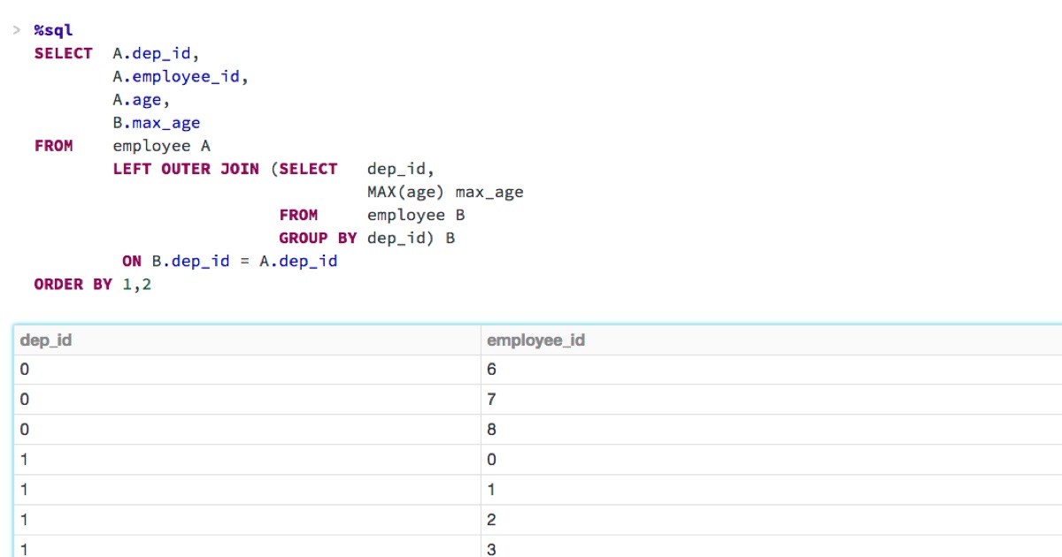
Another very common pattern is using a subquery in the FROM clause. This allows you to treat the result of the subquery as a temporary table, often called a derived table. You must give this derived table an alias.

Correlated Subqueries

A correlated subquery is different: it depends on the outer query for its values. It cannot be run independently. The subquery is executed once for each row processed by the outer query.

This row-by-row execution makes them powerful but potentially slow on large datasets.

Let's watch the next segment of the same video to understand this crucial concept.

Here is the classic example of a correlated subquery shown in the video:

-- Find employees who earn more than the average salary in their own department
SELECT employee_name, salary, department_id
FROM employees e1
WHERE salary > (
  SELECT AVG(salary)
  FROM employees e2
  WHERE e2.department_id = e1.department_id -- Correlation: inner query depends on the outer query's current row
);

For each employee (e1) in the outer query, the inner query recalculates the average salary for that specific employee's department.

2. Common Table Expressions (CTEs)

While subqueries are powerful, they can make your code look nested and complex, especially when you have multiple levels. Common Table Expressions (CTEs) solve this by letting you define temporary, named result sets that you can reference within your main query. They drastically improve the readability and structure of complex SQL.

A CTE is defined using the WITH keyword.

Now, let's see a practical comparison of subqueries and CTEs and explore the advantages of using CTEs.

The key advantages of CTEs are:

1. Readability: Complex logic is broken down into sequential, named steps, making the query flow like a story.
2. Reusability: You can reference the same CTE multiple times within a single SELECT, INSERT, UPDATE, or DELETE statement, avoiding code duplication.
3. Recursion: CTEs can reference themselves, allowing you to query hierarchical data (like organizational charts). This is an advanced topic but a unique capability of CTEs.

3. Hands-On Practice

Time to put this into practice. Let's write some queries in your Databricks workspace.

Instructions:

1. Open the SQL Editor in your Databricks workspace.
2. Ensure you have a SQL Warehouse running and selected.
3. Execute the following code to create a sales_data temporary view.

CREATE OR REPLACE TEMP VIEW sales_data(product_id, category, region, units_sold, unit_price) AS
VALUES
  (1, 'Electronics', 'North America', 120, 900.00),
  (2, 'Electronics', 'Europe', 80, 950.00),
  (3, 'Apparel', 'North America', 300, 45.00),
  (4, 'Apparel', 'Asia', 450, 40.00),
  (5, 'Home Goods', 'Europe', 150, 120.00),
  (6, 'Home Goods', 'North America', 200, 110.00),
  (7, 'Electronics', 'Asia', 100, 850.00);

-- Query the view to see its contents
-- SELECT * FROM sales_data;

Now, write SQL queries to answer the following questions.

Practice Questions:

1. Subquery in WHERE: Find all sales records for products in the 'Electronics' category that sold more units than the overall average number of units sold across all categories. (Hint: Use a scalar subquery).

2. Subquery in FROM (Derived Table): First, calculate the total revenue (units_sold * unit_price) for each sale and the average revenue for its region. Then, join this result back to the original table to show the product_id, category, region, and the calculated total and average revenues for each product.

   • Hint: Your subquery in the FROM clause should calculate AVG(units_sold * unit_price) and group by region.

3. CTE Transformation: Solve the same problem as in question #2, but this time use two CTEs.

   • The first CTE, sales_revenue, should calculate the total revenue for each sale.
   • The second CTE, region_avg_revenue, should use the sales_revenue CTE to calculate the average revenue per region.
   • Finally, join these CTEs in your main query to get the desired result. Notice how much clearer the logic is.

Conclusion

Excellent work! You have now mastered two essential techniques for structuring complex SQL queries. Understanding when and how to use subqueries and CTEs is a hallmark of a proficient data engineer.

Key Takeaways

• Subqueries are queries nested inside another query. They are useful for simple, one-off lookups.
  • Non-correlated subqueries run once and are independent of the outer query.
  • Correlated subqueries run once for each row of the outer query and are dependent on it.
• Common Table Expressions (CTEs) use the WITH clause to create named, temporary result sets. They are the preferred method for complex, multi-step queries because they improve readability, modularity, and allow for reusability within a single statement.
• For most complex transformations, CTEs provide a cleaner and more maintainable structure than deeply nested subqueries.

Next Steps

In our next lesson, we will explore window functions. These are powerful analytical functions that perform calculations across a set of table rows. You will see that CTEs are the perfect tool for preparing or "staging" your data before applying a window function, allowing you to combine these advanced techniques to solve very complex problems.