Pre-registration for Robust Research

1. The Pre-registration Commitment

At its core, a pre-registration is a time-stamped, uneditable document that contains your research plan, including your hypotheses and your complete data analysis strategy. It is typically deposited in a public registry like the Open Science Framework (OSF) before data collection or analysis begins. This act of "calling your shot" prevents the kind of post-hoc rationalization that leads to p-hacking and HARKing (Hypothesizing After the Results are Known).

The video highlights that pre-registration is not about restricting exploration; it's about being transparent about it. You are still free to explore your data, but any findings from unplanned analyses must be labeled as exploratory, signaling to yourself and others that they require independent replication.

2. Crafting a P-hack Proof Analysis Plan

To build our pre-registration, we need a plan that is specific, precise, and exhaustive. A vague plan leaves too many researcher degrees of freedom on the table. We will use the five-point Pre-SPEC framework, developed for clinical trials, to ensure our plan is robust.

Let's now apply the Pre-SPEC framework to our vee relationship experiment.

• (1) Pre-specify before recruitment: We are fulfilling this requirement by designing the plan now, before any data is collected.

• (2) Specify a single primary analysis strategy: This is our most critical decision.

  • Primary Outcome: Our primary dependent variable for confirmatory testing will be the Triadic_Satisfaction composite index, as constructed in the previous module. We will not switch to a sub-scale or a different construct.
  • Primary Hypothesis: We must state our main research question as a single, testable hypothesis. For example: "The 'Nesting' living arrangement will result in a significantly higher mean Triadic_Satisfaction score compared to the average of the two 'Separate' living arrangements ('Partner_A_Separate' and 'Partner_B_Separate')."

• (3 & 4) Plan each aspect with enough detail:

  • Analysis Population: "All data from the triad will be included. Daily data points will be excluded if fewer than 75% of the EMA prompts for that day are completed by all three members."
  • Statistical Model: We must be explicit. Given the nested structure of our data (time points within participants in a single system), a linear mixed-effects model (LMM) is appropriate.
    • Model Specification: Triadic_Satisfaction ~ Living_Arrangement + Period + (1 | Participant_ID)
    • Fixed Effects: Living_Arrangement (our primary predictor, dummy-coded), Period (a numerical variable 1, 2, 3... to control for time trends or sequence effects).
    • Random Effects: A random intercept for Participant_ID (1 | Participant_ID). This is essential as it accounts for the fact that observations from the same person are not independent. Since we have only three participants, we will not model participant-level random slopes.
    • Covariates: No covariates will be included in the primary confirmatory model. This prevents p-hacking via covariate selection. We will list potential covariates (e.g., baseline stress, personality) for pre-specified exploratory models.
  • Missing Data: "Missing data at the item level will be handled within the LMM estimation using Full Information Maximum Likelihood (FIML), under the assumption that data are Missing At Random (MAR)."

• (5) Choices made deterministically:

  • Contrast: The primary hypothesis will be tested using a single, planned contrast: (Nesting) vs. (average of A_Separate, B_Separate).
  • Alpha Level: The threshold for statistical significance for this single primary test will be $\alpha =0.05$, two-tailed.
  • Assumption Violations: "We will visually inspect model residuals for normality and homoscedasticity. If significant heteroscedasticity is observed (e.g., via a Breusch-Pagan test, p < .05), we will re-estimate the model using robust standard errors. No other changes to the model specification will be made based on residual diagnostics."

This level of specificity effectively closes the door on the major researcher degrees of freedom we identified in the last lesson.

3. Taming the Multiple Comparisons Problem

Even with a single primary hypothesis, we are collecting data on multiple outcomes (e.g., individual satisfaction of A, B, and C; dyadic satisfaction scores). If we test our Living_Arrangement intervention on all of them, we run into the multiple comparisons problem: the more tests you run, the higher your chance of finding a "significant" result purely by chance.

The video makes a critical point: the solution isn't just a mathematical formula; it's a logical distinction between confirmatory and exploratory analyses.

Our Multiple Comparisons Strategy

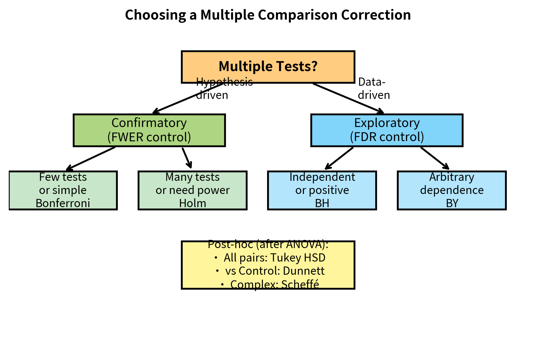
Here is the rule we will specify in our pre-registration plan. It explicitly separates our single confirmatory test from our exploratory analyses.

1. Confirmatory Test (One Test): Our primary hypothesis concerns the effect of Living_Arrangement on the single Triadic_Satisfaction index. Since this is one pre-specified test, no correction for multiple comparisons is needed. We will evaluate it against our $\alpha =0.05$ criterion.

2. Exploratory Tests (A Family of Tests): We will also explore the effect of Living_Arrangement on our secondary outcomes (e.g., satisfaction for Person A, Person B, Person C, Dyad AB, Dyad AC). This constitutes a "family" of related, interchangeable tests. To report these, we must control the error rate.

   • Method Choice: We have several options. The Bonferroni correction is simple (${\alpha }_{new}={\alpha }_{original}/N_{tests}$) and controls the Family-Wise Error Rate (FWER), the probability of making even one false discovery. However, it is highly conservative. A more powerful modern approach is to control the False Discovery Rate (FDR), which is the expected proportion of false discoveries among all reported discoveries. The Benjamini-Hochberg (BH) procedure is the standard method for controlling FDR.
   • Our Rule: "For the family of 5 exploratory tests on individual and dyadic satisfaction outcomes, we will apply the Benjamini-Hochberg procedure to control the False Discovery Rate at q = 0.05. Only effects that are significant after this correction will be interpreted as potentially meaningful exploratory findings."

This two-tiered approach allows us to maintain statistical rigor for our primary claim while still having the power to explore our data for new insights in a principled way.

Conclusion

In this lesson, we have moved from identifying analytical pitfalls to constructing a robust plan to avoid them. By formulating a detailed pre-registration, we make a clear commitment to our primary hypothesis and our analytical strategy, effectively preventing p-hacking and HARKing for our confirmatory claims.

Key Takeaways:

• A pre-registration plan is a time-stamped, uneditable document specifying your hypotheses and analysis plan before seeing the data.
• A robust plan follows the Pre-SPEC principles: it specifies a single primary analysis with enough detail for replication, and all choices are made deterministically.
• For our vee experiment, this means locking in the Triadic_Satisfaction index as the primary outcome and specifying the exact linear mixed-effects model for the analysis.
• The multiple comparisons problem is managed by strictly distinguishing between the single, uncorrected confirmatory test and the family of exploratory tests, for which we will control the False Discovery Rate (FDR).

By creating this plan, we have not only constrained our own researcher degrees of freedom but have also created a public record of our intentions, dramatically increasing the transparency and credibility of our research.

In our next lesson, we will delve deeper into the concept of HARKing (Hypothesizing After the Results are Known). While we've designed our plan to prevent it, the next lesson will explore the nuances of this practice and further solidify the crucial distinction between confirmatory and exploratory mindsets.