Sensitivity Analysis for Unmeasured Confounding

1. The Mechanics of Confounding Bias

At its heart, bias from an unmeasured confounder, $U$, arises from two separate pathways operating simultaneously:

1. The association between the confounder $U$ and the treatment $T$.
2. The association between the confounder $U$ and the outcome $Y$.

If either of these pathways is broken (i.e., the association is zero), $U$ is not a confounder. The bias is a function of the strength of both pathways. We can formalize this idea and see how to estimate the size of the bias.

The video demonstrates that for a simple linear system, the estimated effect is the true effect plus a bias term that depends on the strength of the $U\to T$ and $U\to Y$ paths. Our goal in sensitivity analysis is to work backward: we have an observed (and potentially biased) effect, and we want to know what the true effect would be under different assumptions about the strength of those two confounding pathways.

To do this in a general way, we need a standardized measure for the "strength" of these pathways.

2. Quantifying Confounder Strength with Partial R-squared

While the linear model with its coefficients is intuitive, a more robust and standardized approach is to quantify the strength of associations using partial R-squared ($R^2$). This metric has a clear interpretation that is consistent across different types of variables and models.

This gives us our two key sensitivity parameters:

• Confounder-Outcome Strength ($R_{Y\sim U|\mathbf{X},T}^2$): The percentage of residual variance in the outcome ($Y$) that is explained by the unmeasured confounder ($U$), after controlling for the observed covariates ($\mathbf{X}$) and the treatment ($T$).
• Confounder-Treatment Strength ($R_{T\sim U|\mathbf{X}}^2$): The percentage of residual variance in the treatment ($T$) that is explained by the unmeasured confounder ($U$), after controlling for the observed covariates ($\mathbf{X}$).

With these two parameters, we can now create a sensitivity plot.

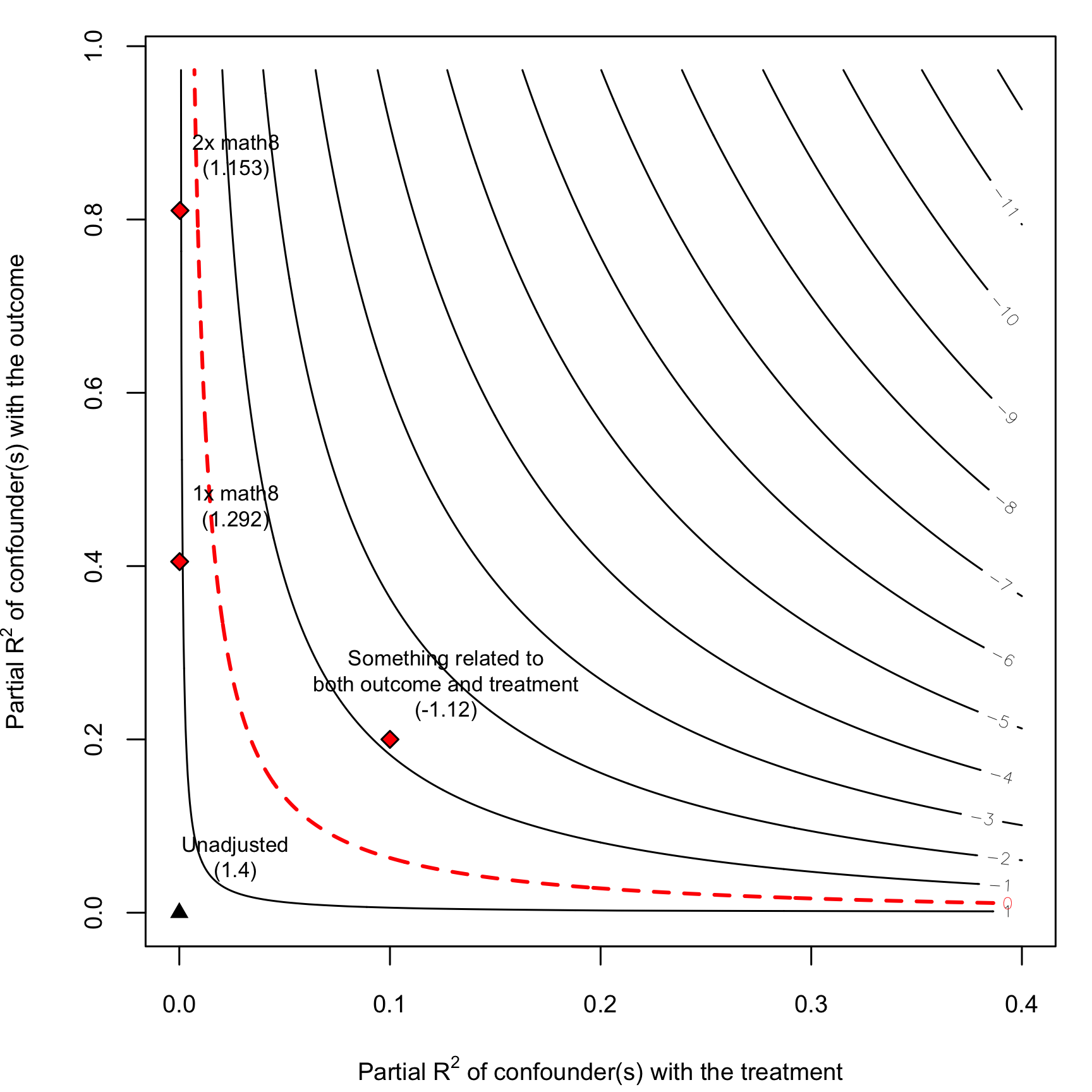
This plot is the core tool of our analysis. The point at (0,0) represents our original, potentially biased estimate, assuming no unmeasured confounding. As we move away from the origin, we are introducing a hypothetical confounder of increasing strength. The contour lines tell us what our estimate would have been in the presence of such a confounder. The red dashed line is critical: any combination of strengths on or beyond this line would be sufficient to "explain away" our result, reducing the estimated effect to zero or flipping its sign.

3. Benchmarking: From Hypothetical to Plausible

The contour plot is powerful, but it presents a universe of hypotheticals. How do we judge what is a "plausible" amount of confounding? Is a partial $R^2$ of 5% large or small? The key is to benchmark the strength of the hypothetical unmeasured confounder against the observed covariates from our model.

This benchmarking step is what makes sensitivity analysis a practical tool rather than a purely abstract exercise. It connects the mathematical what-if scenario to the substantive reality of your research problem.

In the contour plot above, the diamonds labeled "1x math8" and "2x math8" are benchmarks. They represent the strength of a hypothetical confounder that is equally as strong as, or twice as strong as, the observed covariate math8. Since these benchmarks fall well below the tipping point (the red dashed line), we can argue that a confounder would need to be substantially more powerful than math8 to invalidate our conclusion. This adds significant credibility to the result.

4. The E-value: A Common Metric for Sensitivity

Another widely used metric, especially for binary outcomes or risk ratios, is the E-value. It serves a similar purpose to the Robustness Value but is expressed on a different scale.

Definition: The E-value is the minimum strength of association, on the risk ratio scale, that an unmeasured confounder would need to have with both the treatment and the outcome to fully explain away the observed effect. A higher E-value implies greater robustness.

For example, an E-value of 3.0 for an observed risk ratio of 2.0 means that an unmeasured confounder associated with both the treatment and the outcome by a risk ratio of 3.0 each could bring the observed effect to the null (a risk ratio of 1.0).

This plot is interpreted similarly to the partial $R^2$ contour plot. The curves represent tipping points. The green dots (W1) are benchmarks based on observed covariates. The fact that the observed covariates are far from the tipping point curves suggests the result is robust to unmeasured confounding of a similar magnitude.

The concept of identifying the parameters that would "tip" an effect to the null is a general strategy known as a tipping-point analysis.

5. Application to Your Vee-Triad Experiment

Let's ground this in your research project. Imagine you have completed your N-of-1 experiment and found that a particular living arrangement (e.g., living together) has a positive causal effect on your triadic satisfaction index, with an estimated effect size of +0.5 points on a 5-point scale.

Your work isn't done. A skeptic could argue that an unmeasured confounder, like the triad's "baseline level of adventurousness," might explain this finding. Adventurous triads might be more likely to try living together and more likely to report high satisfaction regardless of the arrangement.

To address this, you would conduct a sensitivity analysis:

1. Calculate Robustness Metrics: You compute the Robustness Value (RV) and the E-value for your estimate of +0.5. Let's say the RV is 15%, and the E-value is 3.5.
2. Visualize: You generate contour plots, similar to the ones above, showing the tipping point where the effect would be reduced to 0.
3. Benchmark: You calculate the partial $R^2$ and E-values for your observed covariates (e.g., household income, members' ages, duration of the relationship). Suppose you find that "household income," your strongest observed predictor, has a partial $R^2$ of 4%.
4. Argue and Conclude: You can now make a quantitative argument:

   "Our estimated effect of +0.5 has a Robustness Value of 15%. This means an unmeasured confounder would need to explain at least 15% of the residual variance in both the living arrangement and triadic satisfaction to nullify our finding. For context, our strongest measured covariate, household income, explains only 4% of the variance. Therefore, an unobserved confounder would need to be nearly four times as strong as household income to explain away our results. While such a confounder is theoretically possible, we argue it is substantively implausible, lending credibility to our causal conclusion."

This type of statement is the hallmark of a rigorous and transparent observational or quasi-experimental study.

Conclusion

This lesson has equipped you with one of the most important tools for credible causal inference: sensitivity analysis. You've learned that the assumption of "no unmeasured confounding" doesn't have to be a blind leap of faith. By quantifying how sensitive our results are to violations of this assumption, we can build a much stronger and more nuanced case for our causal claims.

Key Takeaways:

• Sensitivity analysis for unmeasured confounding evaluates how strong the associations between a hypothetical confounder and the treatment/outcome would need to be to alter your conclusion.
• Standardized metrics like partial R-squared, the Robustness Value (RV), and the E-value are used to quantify confounder strength and overall robustness.
• Contour plots are a powerful tool for visualizing the entire space of hypothetical confounding and identifying the "tipping point" where your result would be overturned.
• The most critical step is benchmarking the required strength of a hypothetical confounder against the strength of observed covariates to make a plausibility judgment.

We have now reached the end of our journey through counterfactual reasoning. In our next module, we will pivot to the practical tasks of estimation and synthesis. We will begin by learning how to simulate data from the structural causal model you have designed. This will allow you to test your entire analysis pipeline and understand your model's behavior before you ever collect a single real data point, a crucial step in preparing for a successful experiment.