Necessity vs. Sufficiency in Triadic Living Arrangements

1. The Concepts of Necessity and Sufficiency

Before diving into formal probabilistic definitions, let's build a clear intuition for what "necessary" and "sufficient" mean in a causal context. These terms are used frequently in everyday reasoning, and understanding their logical structure is the first step.

This conceptual framework is the foundation. Now, let's translate these ideas into the rigorous language of counterfactuals, which will allow us to quantify them as probabilities.

2. Formalizing Probabilities of Causation

Judea Pearl's work provides the formal counterfactual semantics for necessity and sufficiency. We will define three key quantities: the Probability of Necessity (PN), the Probability of Sufficiency (PS), and the Probability of Necessity and Sufficiency (PNS).

Let $X$ be a binary treatment variable (e.g., $X=x$ for a specific living arrangement and $X=x^{\prime }$ for the alternative) and $Y$ be a binary outcome (e.g., $Y=y$ for high satisfaction and $Y=y^{\prime }$ for low satisfaction).

Let's summarize and interpret these crucial definitions:

• Probability of Necessity (PN): $\text{PN}\triangleq P(Y_{x^{\prime }}=y^{\prime }|X=x,Y=y)$

  • In words: Given that the triad adopted the arrangement ($X=x$) and achieved high satisfaction ($Y=y$), what is the probability that they would have had low satisfaction ($Y_{x^{\prime }}=y^{\prime }$) had they chosen the alternative arrangement?
  • Interpretation: This measures how essential or indispensable the cause was for the observed outcome. A high PN suggests the outcome was heavily dependent on the cause.

• Probability of Sufficiency (PS): $\text{PS}\triangleq P(Y_x=y|X=x^{\prime },Y=y^{\prime })$

  • In words: Given that the triad did not adopt the arrangement ($X=x^{\prime }$) and has low satisfaction ($Y=y^{\prime }$), what is the probability that they would have had high satisfaction ($Y_x=y$) if they had adopted it?
  • Interpretation: This measures the producing or generating capacity of the cause. A high PS suggests the intervention is a reliable way to produce the outcome in those who currently lack it.

• Probability of Necessity and Sufficiency (PNS): $\text{PNS}\triangleq P(Y_x=y,Y_{x^{\prime }}=y^{\prime })$

  • In words: What is the probability that an individual (or in our case, the triad) is a "responder"—someone who would have high satisfaction under the new arrangement but low satisfaction under the alternative?
  • Interpretation: This captures the proportion of the population for whom the treatment is both necessary and sufficient. It's a measure of individual-level causal response.

To understand how we compute these counterfactual quantities, it helps to visualize the process.

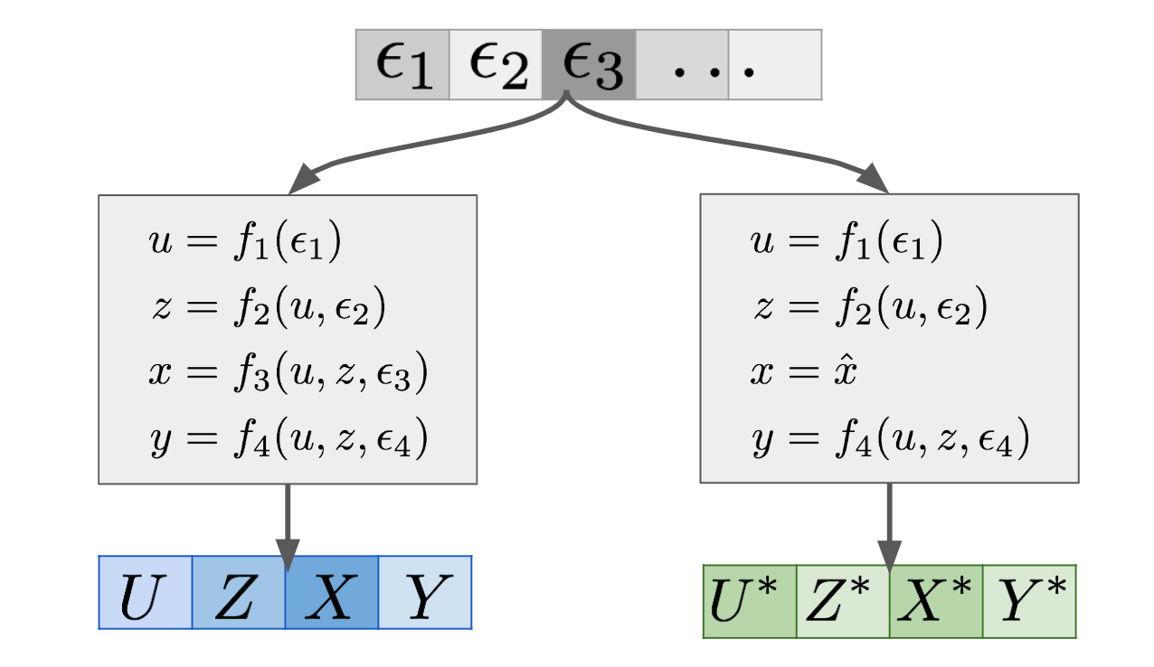
This image shows that to answer a question like "what would Y have been if X had been $x^{\prime }$?", we must hold the state of the world $u$ (represented by the exogenous variables $ϵ$) constant, change the equation for $X$, and re-solve the system. The probabilities PN, PS, and PNS are defined over the distribution of these exogenous factors.

3. Identification: Can We Compute PN and PS from Data?

Defining these quantities is the first step; computing them from experimental data is the next. As with all causal quantities, their identifiability depends on the assumptions we are willing to make.

The Ideal Case: Exogeneity and Monotonicity

Under very strong (and often unrealistic) assumptions, we can calculate a single, exact value for PN, PS, and PNS. The two key assumptions are:

1. Exogeneity: The choice of living arrangement is not confounded. Essentially, it's "as if" it were randomly assigned.
2. Monotonicity: The living arrangement can only help or have no effect; it never hurts. Formally, for any triad, it's impossible that they would have high satisfaction under arrangement $x^{\prime }$ but low satisfaction under $x$.

The reading shows that under these assumptions, the probabilities of causation can be computed directly from observational probabilities:

• $\text{PNS}=P(y|x)-P(y|x^{\prime })$, which you'll recognize as the risk difference.
• $\text{PN}=\frac{P(y|x)-P(y|x^{\prime })}{P(y|x)}$, known as the excess risk ratio or attributable fraction.
• $\text{PS}=\frac{P(y|x)-P(y|x^{\prime })}{1-P(y|x^{\prime })}$.

These formulas provide a powerful bridge from abstract counterfactuals to concrete calculations. However, their validity hinges entirely on the strong, untestable assumptions of exogeneity and monotonicity.

The Realistic Case: Dealing with Unmeasured Confounding

In your vee-triad experiment, exogeneity is unlikely to hold perfectly. Unmeasured factors like personality traits, past relationship history, or financial security could influence both the choice of living arrangement and the resulting satisfaction levels. When such unmeasured confounding exists, we can no longer compute a single value for PN or PS.

Instead, we turn to partial identification. Rather than giving up, we compute bounds—a lower and upper limit for the true value. This provides an honest assessment of what can be learned from the data.

The Tian-Pearl bounds for PNS are derived from the observable probabilities $P(y|x)$ and $P(y^{\prime }|x^{\prime })$. They provide a "worst-case" range for PNS without assuming exogeneity.
The bounds are given by:

This is a profoundly useful result. Even with confounding, we can still constrain our quantity of interest. If the lower bound is greater than zero, we can conclude that the treatment must be a necessary and sufficient cause for at least some fraction of the population.

4. Application to the Vee Triad Experiment

Let's translate this to your project. Imagine you've completed your N-of-1 crossover experiment measuring triadic satisfaction under two arrangements: living together ($X=1$) and living apart ($X=0$). You find the following probabilities from your data:

• $P(Y=1|X=1)=0.8$ (80% of the time, the triad reports high satisfaction when living together)
• $P(Y=1|X=0)=0.3$ (30% of the time, they report high satisfaction when living apart)
• This means $P(Y=0|X=0)=0.7$.

Let's evaluate necessity and sufficiency.

Scenario 1: Assume Exogeneity and Monotonicity (A strong, perhaps naive, assumption for initial analysis)

• PNS = $P(y|x)-P(y|x^{\prime })=0.8-0.3=0.5$.
  • Interpretation: We estimate that for 50% of the time-periods, living together is both necessary and sufficient for the triad's high satisfaction.
• PN = $\frac{0.8-0.3}{0.8}=\frac{0.5}{0.8}=0.625$.
  • Interpretation: On occasions when they were happy living together, there is a 62.5% probability that this arrangement was necessary—that they would have been unhappy otherwise.
• PS = $\frac{0.8-0.3}{1-0.3}=\frac{0.5}{0.7}\approx 0.714$.
  • Interpretation: On occasions when they were unhappy living apart, there is a 71.4% probability that moving in together would be sufficient to make them happy.

Scenario 2: Acknowledge Potential Confounding (A more robust, honest approach)
We cannot assume exogeneity. We must use partial identification to bound the PNS.

• Lower Bound = $\max [0,P(y|x)+P(y^{\prime }|x^{\prime })-1]=\max [0,0.8+0.7-1]=\max [0,0.5]=0.5$.
• Upper Bound = $\min [P(y|x),P(y^{\prime }|x^{\prime })]=\min [0.8,0.7]=0.7$.
• PNS Bounds: $[0.5,0.7]$.

Interpretation: Even without assuming away confounding, our data allow us to conclude that the proportion of time where living together is a necessary and sufficient cause of high satisfaction is between 50% and 70%. The fact that the lower bound is substantially greater than zero provides strong evidence of a robust individual-level causal effect.

Conclusion

In this lesson, we have moved from attributing effects to dissecting the nature of the cause itself. You are now equipped to distinguish between and quantify the necessity and sufficiency of an intervention.

Key Takeaways:

• Necessity (PN) asks if the cause was required for an outcome that occurred, while Sufficiency (PS) asks if the cause would be enough to produce an outcome that is currently absent.
• These concepts are formally defined using counterfactual probabilities over a structural causal model.
• Under the strong assumptions of exogeneity and monotonicity, PN and PS can be calculated as single point estimates from the data.
• In the more realistic presence of unmeasured confounding, we can use partial identification to compute sharp bounds on the Probability of Necessity and Sufficiency (PNS), providing a robust range of plausible values.

This lesson provides a critical tool for interpreting your final experimental results, allowing you to make more nuanced and defensible claims about the causal role of different relationship dynamics. In our next and final lesson of this module, we will address the uncertainty in our assumptions head-on by conducting a sensitivity analysis, where we will formally ask: "Just how strong would an unmeasured confounder have to be to alter our conclusions?"