Modeling Shared Environmental Confounders

1. Confounders: The Source of Spurious Correlation

At its core, a confounder is a common cause of two or more other variables in a system, creating a non-causal "backdoor" path between them. This backdoor path generates spurious correlations, making it difficult to isolate the true causal effect you're interested in.

The book "Causal Inference: The Mixtape" provides a clear introduction to this concept.

In the education example, unobserved "background" (B) is a common cause of both parental education and the child's own education, creating a spurious association between them. In our vee-triad, an unobserved variable like Financial_Stress could be a common cause of each partner's sense of security. If we see that Sec_A and Sec_P are correlated, we cannot immediately conclude that one causes the other; the correlation might be entirely driven by their shared response to financial pressure.

2. Two Flavors of Dependence in Networks

Your background in analyzing complex social systems has undoubtedly shown you that interconnections can arise from different sources. In the context of causal networks, it's useful to formally distinguish between two types of dependence. The first is dependence due to direct transmission, which is what we modeled in the last lesson with our interference arrows (e.g., Partner A's psychological state directly affecting Partner P's outcome).

The second type is latent variable dependence, which is precisely the issue of shared confounding. This arises when individuals who are connected in a network are more likely to share unmeasured traits or be exposed to common environmental factors. The following resource provides an excellent and formal distinction between these two concepts.

As the paper explains, homophily—the tendency for similar people to form ties—is a classic source of latent variable dependence. In our triad, this could manifest if the individuals came from a similar socioeconomic background, which in turn affects their individual stress responses and satisfaction levels. Modeling this requires us to explicitly add nodes for these shared factors.

3. Visualizing Shared Confounders in the Vee-Triad DAG

Let's update our DAG to more explicitly include shared confounders. We will add a measured confounder, Financial Situation (FS), which we assume we can observe (e.g., through surveys on income and savings). We will also retain an unmeasured confounder, Social Stigma (U_Stigma), representing external judgment that affects the triad but is harder to quantify.

A simplified version of our DAG might now look like this:

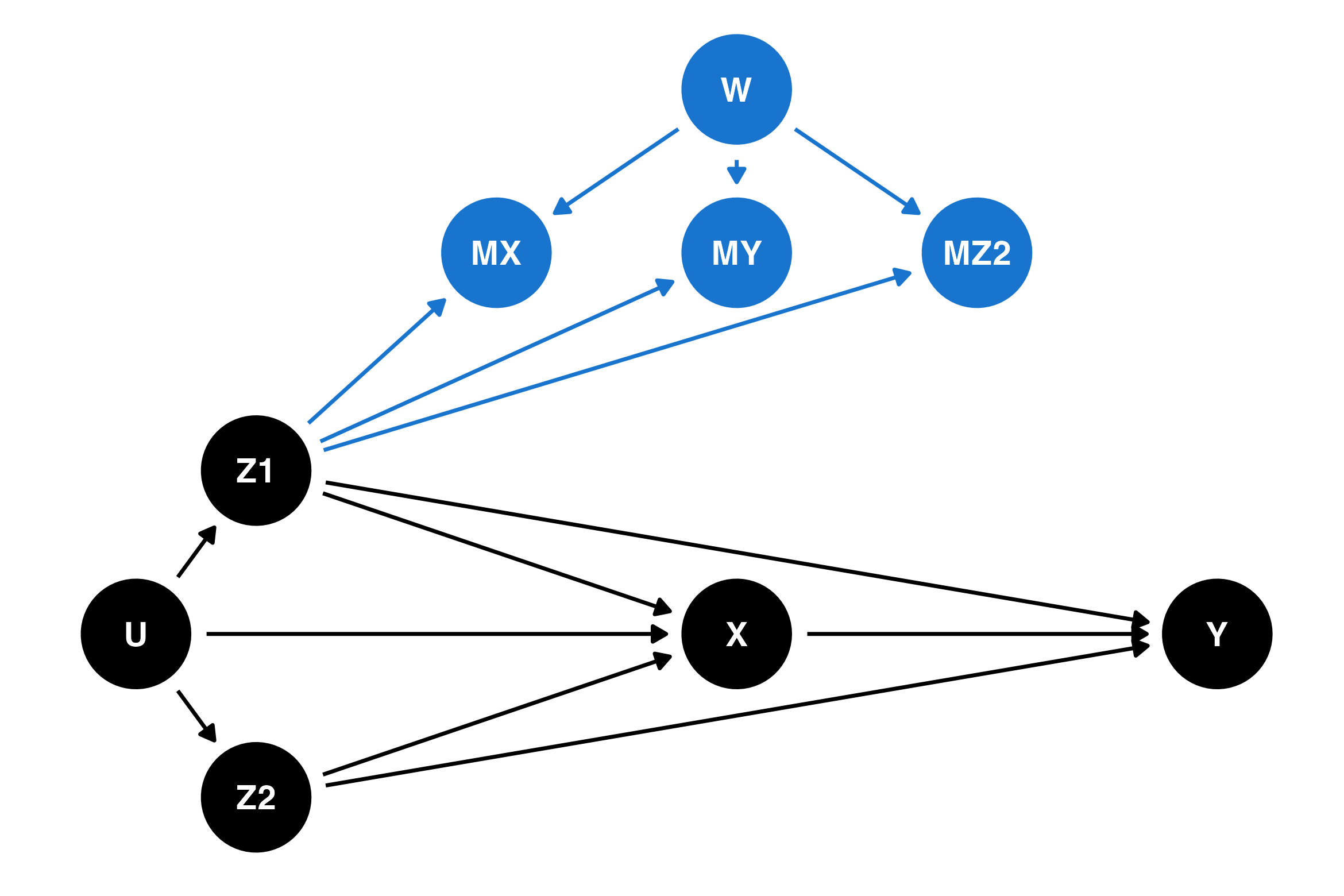
With this graph, the problem becomes clear. Consider the relationship between Partner A's psychological state (MX in the diagram) and Partner B's (MY).

• A naive analysis might find a correlation and assume a causal link.
• However, the shared confounder W (Financial Situation) creates a backdoor path: MX <- W -> MY. This path is non-causal; it simply reflects that both MX and MY are driven by W.

If we fail to account for this path, we will get a biased estimate of how the partners truly influence one another. The solution is to "block" this backdoor path by conditioning on the confounder W. In a statistical model, this means including Financial_Situation as a control variable.

This video gives a good visual review of identifying these paths and satisfying the backdoor criterion.

4. The Challenge of Unobserved Confounders

Conditioning works well for observed confounders like Financial_Situation. But what about unobserved ones like U_Stigma? By definition, we cannot measure and control for them. An unmeasured confounder leaves a backdoor path open, violating a key assumption for causal inference from observational data.

This assumption is often called ignorability or "no unobserved confounding." It states that, conditional on the observed covariates X, the treatment assignment is independent of the potential outcomes. An unobserved common cause violates this directly.

For your project, this is where your qualitative expertise becomes critical. Before finalizing your causal model, you would need to draw on your knowledge of relationship dynamics—and perhaps even interview people in similar relationship structures—to brainstorm all plausible shared factors. Are there shared insecurities? Shared professional pressures? A shared history? Each of these is a potential unmeasured confounder that must be acknowledged. While we can't always control for them, identifying them allows us to perform sensitivity analyses later to test how robust our conclusions are to their potential presence.

5. A Subtle Trap: When Shared Factors are Colliders

Finally, it's crucial to recognize that a shared variable isn't always a confounder. Sometimes, it can be a collider—a variable that is a common effect of two other variables. Conditioning on a collider is a major error that can introduce bias where none existed.

Let's consider a variable in our study: Triad Viability (i.e., whether the triad continues to participate in your long-term study). This is plausibly an effect of each member's satisfaction.

• Partner A's Satisfaction (Y_A) -> Triad Viability
• Partner B's Satisfaction (Y_B) -> Triad Viability

Here, Triad Viability is a collider on the path Y_A -> Triad Viability <- Y_B. If you decide to analyze only the data from triads that "survived" the whole study, you are conditioning on this collider. This will create a spurious statistical association between Y_A and Y_B, potentially leading you to incorrectly conclude that the partners' satisfaction levels are causally linked (or linked in a way they are not).

This is a subtle but common form of selection bias. "The Mixtape" offers a powerful real-world example of this problem.

Conclusion

In this lesson, we have moved from a simple representation of interference to a more robust causal model that accounts for the complexities of the environment surrounding the triad.

Key Takeaways:

• Shared-environment confounders are common causes that affect multiple members of the triad simultaneously, creating non-causal backdoor paths.
• In network science, this is known as latent variable dependence, and it is a distinct source of correlation from direct transmission (interference).
• The primary method for dealing with observed confounders is to condition on them (i.e., control for them in your analysis) to block the backdoor paths they create.
• Unobserved confounders violate the critical "ignorability" assumption. While they cannot be controlled for directly, identifying them through domain expertise is essential for understanding the limitations of a model and planning for sensitivity analyses.
• Be cautious not to condition on colliders (shared effects), such as relationship stability or continued participation in a study, as this can introduce selection bias.

We now have a much more complete DAG for our vee-triad, one that accounts for both interference and confounding. In our next lesson, we will enrich this model further by focusing on the specific mechanisms of change. We will investigate how the living arrangement causally influences satisfaction through mediating psychological states like security and autonomy, addressing the learning outcome: Represent mediating pathways from living arrangement through psychological mechanisms to satisfaction.