Simpson's Paradox in Satisfaction Data

1. The Paradox of Aggregation

At its core, Simpson's paradox is a statistical illusion. It occurs when a trend that appears in different groups of data disappears or reverses when these groups are combined. What might look like a positive association in the total population could, in fact, be a negative association within every single subgroup.

To build an initial intuition, let's watch a video from Dr. Trefor Bazett that uses real-world data on COVID-19 fatality rates to illustrate this phenomenon with remarkable clarity.

The key takeaway is that an unobserved variable—in this case, the age distribution of patients in each country—can create a misleading trend in the aggregated data. This "lurking" variable is what we, in causal inference, would label a confounder.

The image below shows the classic visual signature of the paradox. When all the data points are pooled together (ignoring the colors), the overall trend line (in blue) slopes downward. However, within each subgroup (distinguished by color), the trend is clearly upward.

2. The Causal Story: Why It Happens

The paradox is resolved by moving from a purely statistical description to a causal explanation. The decision of whether to trust the aggregated or the subgroup-specific results is not a statistical choice—it is a causal one, determined entirely by the underlying causal structure of the problem.

This is where your knowledge of Directed Acyclic Graphs becomes essential. Let's watch another video, this time from Brady Neal's "Causal Inference" course, which uses DAGs to dissect the paradox.

As the video makes clear, Simpson's paradox often arises from a classic confounding structure. Consider the case where the grouping variable, let's call it $Z$, is a common cause of both the treatment $T$ and the outcome $Y$.

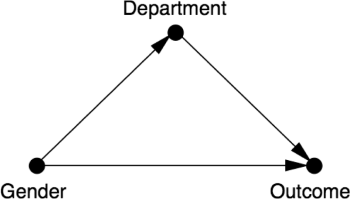
In this structure, $Z\to T$ and $Z\to Y$. When you analyze the relationship between $T$ and $Y$ by aggregating all data, you are ignoring $Z$. This leaves the "backdoor path" $T\leftarrow Z\to Y$ open, and the observed association between $T$ and $Y$ becomes a mix of the true causal effect and spurious correlation from the confounder $Z$. By analyzing the data within each level of $Z$, you are effectively "blocking" this backdoor path, isolating the true effect of $T$ on $Y$.

This distinction is not merely academic; it is the fundamental challenge of causal analysis in non-experimental data. The following commentary provides a sharp perspective on this, arguing that these paradoxes are not statistical curiosities but direct consequences of trying to infer causation without causal reasoning.

The paper's central message is that statistics alone cannot tell you whether to adjust for a third variable. Only your background knowledge, encoded in a DAG, can guide that decision.

3. Simpson's Paradox in the Vee-Triad Experiment

Now, let's apply this to your study. How could you be misled by Simpson's paradox when analyzing the satisfaction data from the vee-triad?

Imagine you are testing the effect of a specific intervention, let's say a new communication protocol (T), on individual satisfaction (Y). You collect satisfaction data from all three members of the triad: the Pivot (A), Partner B, and Partner C.

It's tempting to pool all the data together to increase your statistical power and get one overall estimate of the protocol's effect. However, the role of the person in the triad (Pivot, Partner B, or Partner C) could be a powerful confounder.

Let's construct a plausible causal story that would produce the paradox:

1. Causal Structure: The person's Role (Z) is a common cause of both their likelihood of adopting the Communication Protocol (T) and their baseline Satisfaction (Y). The DAG is $T\leftarrow Z\to Y$, with a direct arrow $T\to Y$ representing the true causal effect we want to estimate.

2. Plausible Mechanism:

   • $Z\to Y$: Let's assume the Pivot's role carries more inherent stress and responsibility. Consequently, the Pivot might have a lower baseline level of satisfaction compared to Partners B and C, independent of any specific communication protocol.
   • $Z\to T$: As the central figure managing two relationships, the Pivot might be more motivated to adopt and rigorously follow the new communication protocol than the other partners. Thus, the Pivot has a higher probability of being in the "treatment" group.
   • $T\to Y$: Let's assume the protocol is genuinely effective. For any given person, adopting the protocol increases their satisfaction.

3. The Paradoxical Result:

   • When you analyze the data within each role, you find that the communication protocol is associated with higher satisfaction for the Pivot, for Partner B, and for Partner C. The effect is positive in all three subgroups.
   • However, when you aggregate the data, you are combining a group (Partners) with high baseline satisfaction and low treatment uptake with another group (the Pivot) with low baseline satisfaction and high treatment uptake.
   • The resulting aggregated data could show that individuals who used the protocol (who are disproportionately the lower-satisfaction Pivot) have, on average, lower satisfaction than those who did not (who are disproportionately the higher-satisfaction Partners). This would lead to the dangerously incorrect conclusion that the communication protocol is harmful.

To avoid this, your causal model and analysis plan must explicitly account for Role as a confounder. In statistical terms, this means not running a simple pooled regression of Satisfaction ~ Protocol. Instead, you would need a model that includes Role as a covariate, effectively estimating the effect of the protocol conditional on role.

The following resource shows exactly how this is done in a Bayesian modeling context, contrasting a naive pooled model with a more appropriate unpooled or hierarchical model that accounts for the grouping variable.

This practical example solidifies the link between the causal DAG and the statistical model required to get the right answer. The choice of model is dictated by the arrows in your graph.

Conclusion

This lesson has demonstrated that Simpson's paradox is more than a statistical curiosity; it is a fundamental challenge in causal inference that arises from naive data aggregation. The paradox serves as a powerful reminder that correlation is not causation and that statistical associations can be deeply misleading without a guiding causal model.

Key Takeaways:

• Simpson's Paradox: A trend observed in aggregated data can disappear or reverse when the data is disaggregated into subgroups.
• Causal Explanation: The paradox is typically caused by a confounding variable that is correlated with both the treatment and the outcome. Aggregating the data is equivalent to ignoring the confounder, leading to biased estimates.
• DAGs are Key: The decision to analyze data in aggregate or by subgroup is a causal one. The correct approach is determined by the underlying causal structure, which should be explicitly represented in a DAG.
• Application to Triad: In your experiment, aggregating satisfaction data across different roles (Pivot, Partner B, Partner C) or dyads without proper adjustment could produce a Simpson's paradox, as Role is likely a confounder influencing both behavior and satisfaction.

In our next lesson, we will begin the final module on causal identification. Armed with our detailed structural causal model—now fortified against pitfalls like aggregation bias—we will explore how to use the rules of do-calculus to formally determine whether the causal effects you care about can be estimated from the data you plan to collect.