Gauge Fields and Covariant Derivatives from Local U(1) Invariance

The Geometric Analogy: Derivatives and Parallel Transport

Before diving into the algebra, let's build an intuition based on a concept you are familiar with from your study of General Relativity: differentiating vectors on a curved manifold.

On a flat plane, subtracting two vectors at different points is straightforward because the basis vectors are the same everywhere. On a curved surface, like a sphere, the tangent space at each point is different. You cannot simply subtract a vector at point $p$ from a vector at a nearby point $p+d\mathbf{x}$ because they live in different vector spaces. To make a meaningful comparison, you must first parallel transport the vector from $p$ to $p+d\mathbf{x}$ along the connecting path. The covariant derivative is then the difference between the actual vector at $p+d\mathbf{x}$ and the parallel-transported version of the vector from $p$.

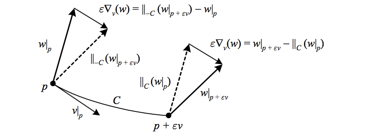
The situation with local gauge symmetry is perfectly analogous. A local U(1) transformation $\psi (x)\to e^{iq\alpha (x)}\psi (x)$ attaches a different "internal" phase reference frame at each spacetime point $x$. Just as we need a connection to compare vectors in different tangent spaces in GR, we need a "gauge connection" to compare the phase of a field at $x$ with its phase at $x+dx$. The gauge field, $A_{\mu }$, will play the role of this connection.

The Comparator and the Covariant Derivative

Let's formalize this idea of parallel transport for our U(1) phase symmetry. We need a way to compare $\psi (x)$ and $\psi (y)$ that respects the local gauge freedom. This requires an object, a "comparator" or "parallel transporter" $U(y,x)$, that connects the internal space at point $x$ to the internal space at point $y$.

The following reading develops this idea from first principles, showing how the definition of a well-behaved derivative in the presence of local symmetry naturally leads to the introduction of a gauge field.

The key insight from this reading is that by demanding a derivative that transforms simply under local phase rotations, we are forced to introduce a new entity, the vector gauge field $A_{\mu }(x)$, which acts as an infinitesimal parallel transporter. The final form, $D_{\mu }\psi =({\partial }_{\mu }+ie{A}_{\mu })\psi$, shows that the covariant derivative is the ordinary derivative plus a correction term involving this new field. The transformation rule for the gauge field, $A_{\mu }\to A_{\mu }-\frac{1}{e}{\partial }_{\mu }\alpha$, is precisely what is needed to make the whole structure work.

An Algebraic Derivation

The "comparator" approach provides excellent physical intuition. Now, let's re-derive the same result using a more direct algebraic method common in QFT literature. This approach is less about building from infinitesimal transport and more about enforcing a desired algebraic transformation property on the derivative operator itself.

We start by postulating the form of the covariant derivative, $D_{\mu }={\partial }_{\mu }-i{A}_{\mu }$, where we treat $A_{\mu }$ as an unknown gauge field. (Note the different sign convention; this is a matter of definition). We then demand that the operator $D_{\mu }$ as a whole transforms in a way that preserves the covariance of $D_{\mu }\psi$.

This operator-based derivation beautifully complements the comparator approach. It shows that if we want $D_{\mu }\varphi$ to transform like $\varphi$ (i.e., picking up a factor of $e^{i\alpha }$), the operator $D_{\mu }$ itself must transform "in the adjoint representation" of the gauge group. Working this out leads to the same transformation for the gauge field we found earlier:

and confirms the form of the covariant derivative:

The lecture in the following video walks through this same derivation, providing a dynamic explanation that ties the pieces together.

At the end of this segment, the lecturer correctly identifies the transformation of $A_{\mu }$ as the familiar gauge transformation from electromagnetism. By demanding local phase invariance for a charged field, we have been forced to invent a vector field that transforms exactly like the electromagnetic four-potential.

The Deeper Picture: Gauge Fields as Connections on Fiber Bundles

The analogy between the covariant derivative in GR and the gauge covariant derivative is not merely a pedagogical tool; it reflects a deep, underlying mathematical unity. Both theories are described by the geometry of fiber bundles. In this framework, the gauge field $A_{\mu }$ is the local representation of a connection one-form on a principal bundle.

This is a highly abstract and mathematically advanced topic, but given your background, it is valuable to see how the concepts we've developed physically are realized in their full geometric glory. The following optional video gives a glimpse into this formalism.

Conclusion

In this lesson, we have taken the crucial step from identifying a problem (the failure of local invariance) to constructing the solution. We have derived the fundamental tools of gauge theory from the ground up by demanding that the laws of physics respect a local symmetry.

Key Takeaways:

• The problem of differentiating fields under local gauge transformations is analogous to differentiating vectors on a curved manifold. Both require a connection to enable parallel transport.
• The covariant derivative, $D_{\mu }$, is a modified derivative that transforms covariantly under gauge transformations, meaning $(D_{\mu }\psi {)}^{\prime }$ transforms just like ${\psi }^{\prime }$.
• To achieve this, we must introduce a gauge field (or gauge connection) $A_{\mu }$. For a U(1) symmetry where a field transforms as $\psi \to e^{iq\alpha (x)}\psi$, the covariant derivative and gauge field are:
  • $D_{\mu }={\partial }_{\mu }-iq{A}_{\mu }$
  • $A_{\mu }(x)\to A_{\mu }^{\prime }(x)=A_{\mu }(x)+{\partial }_{\mu }\alpha (x)$
    (Note: conventions for the sign and placement of the charge $q$ can vary, but the underlying structure is the same).
• The gauge field $A_{\mu }$ we were forced to introduce has exactly the transformation properties of the electromagnetic four-potential.

We now have the necessary machinery. We have a derivative, $D_{\mu }$, that behaves properly under local gauge transformations. In our next lesson, we will replace the problematic ordinary derivative ${\partial }_{\mu }$ with our new covariant derivative $D_{\mu }$ in the Dirac Lagrangian. We will see that this simple replacement not only restores gauge invariance but also automatically generates a new term in the Lagrangian—the interaction term between the electron and the photon, which is the foundation of Quantum Electrodynamics (QED).