Chiral Symmetry and the Chiral Anomaly

Chirality and Chiral Symmetry

To begin, we need to carefully distinguish two concepts that are often used interchangeably for massless particles but are fundamentally different: helicity and chirality.

• Helicity is a physical, observable property: the projection of a particle's spin onto its direction of momentum. A right-handed particle has its spin aligned with its momentum, while a left-handed particle has its spin anti-aligned. For a massive particle, you could always "outrun" it by boosting to a reference frame moving faster than the particle, causing its momentum vector to flip and thus reversing its helicity.
• Chirality, on the other hand, is a more abstract, intrinsic property of a particle's wavefunction, related to how it transforms under the Lorentz group. It is a fundamental label, much like mass or charge.

For massless particles, which travel at the speed of light, you can never outrun them. Consequently, their helicity is frame-invariant. It turns out that for these particles, the concepts of chirality and helicity coincide.

The following video provides a clear explanation of these two concepts and their relationship.

As the video explains, chirality is associated with the transformation properties of fermion fields. A four-component Dirac spinor $\psi$ can be decomposed into its left-chiral and right-chiral components using the projection operators:

The resulting two-component objects, ${\psi }_L=P_L\psi$ and ${\psi }_R=P_R\psi$, are known as Weyl spinors. The full Dirac spinor is their sum: $\psi ={\psi }_L+{\psi }_R$.

Now, consider the Lagrangian for a single massless Dirac fermion:

Using the properties of the gamma matrices, we can rewrite this Lagrangian in terms of the Weyl spinors:

Notice that the Lagrangian splits into two completely independent pieces, one for the left-chiral field and one for the right-chiral field. There are no terms that mix ${\psi }_L$ and ${\psi }_R$. This separation implies that the Lagrangian is invariant under independent phase rotations of the left- and right-chiral fields:

This is a $U(1{)}_L\times U(1{)}_R$ global symmetry. It's often more convenient to reparametrize these two transformations into their sum and difference:

1. Vector Symmetry $U(1{)}_V$: When ${\alpha }_L={\alpha }_R=\alpha$, the full Dirac spinor transforms as $\psi \to e^{i\alpha }\psi$. By Noether's theorem, this leads to the conservation of the vector current $j_V^{\mu }=\bar{\psi }{\gamma }^{\mu }\psi$, which corresponds to the conservation of fermion number.
2. Axial-Vector (or Axial) Symmetry $U(1{)}_A$: When ${\alpha }_L=-{\alpha }_R=\beta$, the transformation is $\psi \to e^{i\beta {\gamma }_5}\psi$. This is the chiral symmetry. The corresponding Noether current is the axial current, $j_A^{\mu }=\bar{\psi }{\gamma }^{\mu }{\gamma }_5\psi$.

Classically, we expect the axial current to be conserved, ${\partial }_{\mu }{j}_A^{\mu }=0$, just like the vector current. However, as we will now see, this classical expectation is violated by quantum effects.

It's important to note that a mass term, ${\mathcal{L}}_m=-m\bar{\psi }\psi =-m({\bar{\psi }}_R{\psi }_L+{\bar{\psi }}_L{\psi }_R)$, explicitly couples the left- and right-chiral components, breaking the axial $U(1{)}_A$ symmetry. Therefore, chiral symmetry is fundamentally a property of massless fermions.

The Chiral Anomaly: A Quantum Violation

The chiral anomaly is the statement that even for massless fermions, the axial current is not conserved in the quantum theory when the fermions are coupled to a gauge field. This is not because of a flaw in Noether's theorem, but because one of its hidden assumptions—that the quantum measure is symmetric—fails.

To build intuition for this surprising result, it's helpful to look at how it manifests in physical situations. The following reading from David Tong's QFT lecture notes provides two beautiful, intuitive arguments.

Let's summarize the key insights from these arguments:

• The 1+1D Dirac Sea: In 1+1 dimensions, left- and right-chiral fermions are simply left- and right-moving particles. When an electric field is applied, it exerts a force on all charged particles, including those in the infinite negative-energy Dirac sea. This force shifts the momentum of all states, effectively "pulling" particles out of the sea at one end and creating holes (antiparticles) at the other. The result is the creation of, for example, a right-moving particle and a left-moving antiparticle. The total number of fermions is conserved, but the number of right-movers minus the number of left-movers is not. Axial charge is not conserved because the infinite nature of the Dirac sea acts as an inexhaustible reservoir.

• The 3+1D Landau Levels: In 3+1 dimensions, a similar effect occurs in the presence of parallel electric ($\mathbf{E}$) and magnetic ($\mathbf{B}$) fields. The magnetic field quantizes the motion of charged fermions in the plane perpendicular to $\mathbf{B}$ into Landau levels. The lowest Landau level is special: its states are chiral, moving in only one direction along the magnetic field line (e.g., right-movers). This effectively reduces the problem to a 1+1 dimensional system along $\mathbf{B}$. The parallel electric field then accelerates these chiral modes, creating a net flow of axial charge, just as in the 1+1D case.

This latter picture has a stunning realization in condensed matter physics. In materials known as Weyl semimetals, the electronic band structure features points (Weyl nodes) where conduction and valence bands touch. These nodes come in pairs of opposite chirality. They act as the endpoints of the fermion spectrum, analogous to the left- and right-moving sectors in the 1+1D model.

As shown in the image above, applying parallel electric and magnetic fields pumps electrons between Weyl nodes of opposite chirality. This "chiral pumping" is a measurable transport signature of the chiral anomaly, demonstrating how a concept from high-energy physics finds a direct analogue in a material system.

Origin of the Anomaly: Triangle Diagrams and the Path Integral

Having built some physical intuition, we now ask: where does the non-conservation come from mathematically? There are two primary perspectives on this.

1. The Perturbative View: Triangle Diagrams

Historically, the anomaly was discovered by Stephen Adler, John Bell, and Roman Jackiw (ABJ) when performing a perturbative calculation in quantum electrodynamics. They calculated the one-loop Feynman diagram for the divergence of the axial current coupled to two photons.

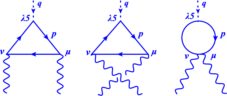
Naively, the calculation seemed to contain ambiguities depending on how one regulated the divergent loop integral. However, they realized that if one insists on preserving the gauge symmetry associated with the vector currents (i.e., the photons), the axial symmetry is necessarily broken. The calculation consistently yields a non-zero value for the divergence of the axial current. The video below briefly introduces this idea.

2. The Non-Perturbative View: Fujikawa's Method

A deeper and more general understanding comes from the path integral formulation of quantum field theory. As you know from your QFT course, quantum transition amplitudes are calculated by summing over all possible field configurations, weighted by $e^{iS/\hslash }$, where $S$ is the classical action.

The crucial insight, due to Kazuo Fujikawa, is that while the classical action $S$ may be invariant under a chiral transformation, the integration measure $\mathcal{D}\psi \mathcal{D}\bar{\psi }$ in the path integral is not. A chiral transformation induces a non-trivial Jacobian factor in the measure. When carefully calculated using a gauge-invariant regularization scheme, this Jacobian precisely accounts for the anomalous term.

The derivation is quite technical, but the conceptual point is paramount: the anomaly arises because the symmetry of the classical action is not a symmetry of the full quantum theory (action + measure).

Both the perturbative and non-perturbative calculations yield the same famous result for the anomalous Ward identity:

where $F_{\mu \nu }$ is the electromagnetic field strength tensor. This equation is the mathematical statement of the chiral anomaly. The $\mathbf{E}\cdot \mathbf{B}$ term beautifully recovers the intuition we built from the Landau level picture.

As the notes mention, this result is connected to the Atiyah-Singer index theorem, a deep result in mathematics that relates the topology of the gauge field configuration to the spectrum of the Dirac operator. This connection explains why the anomaly formula is exact—it receives no further corrections from higher-order loops.

Physical Consequence: The Decay of the Neutral Pion

The chiral anomaly is not just a mathematical subtlety; it explains a crucial physical process: the decay of the neutral pion into two photons, ${\pi }^0\to \gamma \gamma$.

In the theory of the strong force, QCD, the up and down quarks are nearly massless. This gives rise to an approximate chiral symmetry. This symmetry is spontaneously broken (a topic we will explore in the next module), and the pions are the (nearly) massless Goldstone bosons that emerge.

Symmetry arguments based on the classical theory predict that the decay ${\pi }^0\to \gamma \gamma$ should be forbidden. Yet, it is the primary decay mode of the ${\pi }^0$. The resolution is the chiral anomaly. The axial current associated with the ${\pi }^0$ has an ABJ anomaly when coupled to electromagnetism. This anomaly provides the exact mechanism that allows the decay to happen. In fact, the calculation of the decay rate from the anomaly was one of the early triumphs of QCD, as it correctly predicted the rate only if quarks come in three "colors."

Conclusion

In this lesson, we have journeyed from the classical definition of chiral symmetry to its surprising violation at the quantum level. We've seen how this violation, the chiral anomaly, is not a mistake but a deep and predictive feature of quantum field theory.

Key Takeaways:

• Chiral Symmetry: A classical symmetry of the massless Dirac Lagrangian, corresponding to independent phase rotations of the left- and right-chiral components of the fermion field.
• Chiral Anomaly: The quantum-mechanical breaking of the classical axial symmetry. The axial current is not conserved in the quantum theory when coupled to gauge fields.
• Physical Intuition: The anomaly can be visualized as the pumping of fermions between chiral sectors, either in the 1+1D Dirac sea or among the chiral Landau levels in 3+1D. This has a direct analogue in the "chiral pumping" effect in Weyl semimetals.
• Mathematical Origin: The anomaly arises from the non-invariance of the fermionic path integral measure under chiral transformations (Fujikawa's method) or, equivalently, from specific one-loop triangle diagrams in perturbation theory (the ABJ anomaly).
• Physical Consequences: The anomaly is a real physical effect, responsible for processes like the decay of the neutral pion (${\pi }^0\to \gamma \gamma$) that would otherwise be forbidden.

Preview of the Next Module:

The chiral anomaly represents one way a symmetry can be broken: at the quantum level. In our next module, we will explore a completely different, yet equally profound, mechanism: spontaneous symmetry breaking. This occurs when the underlying laws of physics possess a symmetry, but the system's ground state (or vacuum) does not. This is the phenomenon responsible for ferromagnetism, superconductivity, and, most famously, the generation of particle masses via the Higgs mechanism in the Standard Model.