Homotopy Groups and Topological Classification

Introduction

In our previous lesson, we established a crucial connection between symmetry and the macroscopic structure of matter. We saw that when a system undergoes spontaneous symmetry breaking, it settles into one of many degenerate ground states, which together form the order parameter space (or vacuum manifold), $M$ . We ended with a preview of how the "shape" of this space—whether it has holes or other non-trivial features—determines the existence of stable topological defects.

This lesson provides the mathematical language to describe that "shape" precisely. We will introduce homotopy groups, denoted $π_{n} (M)$ , a powerful tool from algebraic topology. These groups classify the different ways one can map spheres of various dimensions into a topological space. As we will see, this abstract-sounding concept has a direct physical interpretation: it classifies the possible "twisted" configurations of the order parameter field, which are the very essence of topological defects. We will begin by building a strong geometric intuition for these groups before solidifying the concepts with more formal definitions.

Homotopy: The Art of Continuous Deformation

At its heart, topology is the study of properties that are preserved under continuous deformations. The central idea for our purpose is that of homotopy, which formalizes the notion of deforming one mathematical map into another.

Topology and geometry for physicists

This document provides a concise mathematical introduction to the core concepts. We'll start with the fundamental definition of homotopy itself.

Please read the definition of homotopy provided in section 1.1. Focus on the passage from the definition. The key is to think of the parameter t in the homotopy function H(x,t) as "time," which smoothly deforms the initial map f(x) into the final map g(x).

Two maps are said to be homotopic if one can be continuously transformed into the other. This relationship partitions all possible continuous maps between two spaces, $X$ and $Y$ , into distinct homotopy classes. A homotopy class consists of all maps that are mutually deformable into one another. The set of these classes tells us about the topological structure of the spaces involved. Homotopy groups are the tools we use to study these classes.

The Fundamental Group, $π_{1} (X)$ : Classifying Loops

The most intuitive homotopy group, and arguably the most important for many physical systems, is the fundamental group, $π_{1} (X)$ . It answers the question: how many fundamentally different ways can you draw a closed loop in a space $X$ ?

A loop that can be continuously shrunk to a point is considered "trivial." A loop that gets snagged on a "hole" in the space is "non-trivial." The fundamental group classifies all the non-equivalent ways a loop can be non-trivial. The following video provides a superb visual introduction to this idea.

A Sphere is a Loop of Loops (Visualizing Homotopy Groups)

This video by Dennis Sweeney, titled "A Sphere is a Loop of Loops", uses excellent animations to build geometric intuition for homotopy groups.

Please watch the first part of the video, which focuses on \pi_1, from this segment. Pay close attention to: How loops are classified by a "winding number" for a space with a hole (the circle, S^1). Why all loops are trivial (can be shrunk to a point) in a space without a hole (the disk, D^2) or on the surface of a sphere (S^2). The concept of a group operation (concatenating loops) and why the order matters for some spaces (the figure-8 example).

As the video illustrates, the fundamental group captures the one-dimensional "hole" structure of a space.

For the circle, $M = S^{1}$ (the order parameter space for a superfluid), loops are classified by an integer winding number $n$ , which counts how many times the loop wraps around the circle. The group operation is addition of winding numbers. Thus, $π_{1} (S^{1}) = Z$ .

Loops on a circle are classified by an integer winding number. A loop wrapping once corresponds to $+1$, twice to $+2$, and so on. These distinct homotopy classes are the elements of the fundamental group $\pi_1(S^1) = \mathbb{Z}$.

For a disk or any space that is simply connected (has no one-dimensional holes), any loop can be shrunk to a point. There is only one homotopy class, the trivial one. The group has only one element, the identity. We write $π_{1} (D^{2}) = {0}$ or $π_{1} (S^{2}) = {0}$ .

Let's now ground this intuition with the formal structure.

Topology and geometry for physicists

We now return to the notes by Emanuel Malek to see the formal definitions corresponding to the video's animations.

Please read Section 2.1, "First homotopy group". This section formalizes the concepts of a loop, the product of loops, and homotopy of loops. It then proves that the set of homotopy classes forms a group, \pi_1(X, x_0), and shows that for path-connected spaces (which all of our physical examples will be), this group is independent of the chosen basepoint x_0.

The key takeaway is that $π_{1} (X)$ is a group whose elements are equivalence classes of loops in the space $X$ . The group operation is loop concatenation. The existence of a non-trivial fundamental group, like $π_{1} (S^{1}) = Z$ , is the topological signature of a one-dimensional hole and, as we'll see, is the condition for the existence of stable line defects (vortices or cosmic strings).

Higher Homotopy Groups, $π_{n} (X)$ : Classifying Spheres

The fundamental group detects holes that can be encircled by a 1D loop. To detect higher-dimensional topological features, like the "emptiness" inside a sphere, we need to probe the space with higher-dimensional objects. This leads to the higher homotopy groups, $π_{n} (X)$ .

The $n$ -th homotopy group, $π_{n} (X)$ , is defined as the set of homotopy classes of maps from an $n$ -dimensional sphere, $S^{n}$ , into the space $X$ .

$π_{1} (X)$ classifies maps of $S^{1}$ (a circle) into $X$ .
$π_{2} (X)$ classifies maps of $S^{2}$ (a sphere) into $X$ .
$π_{3} (X)$ classifies maps of $S^{3}$ (a 3-sphere) into $X$ .
And so on.

The intuition for $π_{2}$ is less immediate than for $π_{1}$ , but the same video provides an excellent analogy.

A Sphere is a Loop of Loops (Visualizing Homotopy Groups)

Let's continue with Dennis Sweeney's visual explanation.

Watch the next major segment on \pi_2, from this point. He masterfully explains \pi_2 in several ways: As "loops of loops". As "swinging a jump rope" or a "butterfly net". As maps from a square with its boundary collapsed to a point, which is topologically an S^2. Focus on why \pi_2(S^2) = \mathbb{Z} (you can wrap a sphere around another sphere an integer number of times) and why \pi_2(S^1) = \{0\} (you can't trap a 2D surface in a 1D space).

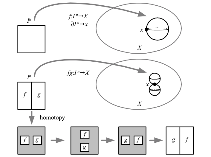
A crucial difference emerges with the higher groups. While the fundamental group $π_{1}$ can be non-abelian (as seen in the figure-8 example), all higher homotopy groups are abelian.

Theorem: For $n \geq 2$ , the group $π_{n} (X)$ is always abelian.

The video gives the intuition for this: when you have at least two dimensions to work with ( $S^{2}$ or higher), two separate "wraps" can slide past each other. This is impossible for one-dimensional loops on a line, which is why $π_{1}$ can be non-abelian.

The formal definition of $π_{n}$ and the proof of this property are found in Malek's notes.

Topology and geometry for physicists

This section generalizes the definitions from \pi_1 to \pi_n.

Please read Section 2.3, "Higher homotopy groups". This section defines an n-loop (as a map from an n-cube I^n with its boundary identified to a point) and the group structure. Pay special attention to Figure 12 and the accompanying text, which provides the diagrammatic proof for why \pi_n is abelian for n > 1.

A visual proof of why $\pi_n$ is abelian for $n \ge 2$. The product of two n-loops, $f$ and $g$, is defined by composing them along one dimension (e.g., $t_1$). For $n \ge 2$, there is at least one other dimension (e.g., $t_2$) available. The maps can be homotopically shrunk to occupy only a part of the cube, allowing them to "slide" past each other in the unused dimension, demonstrating that $f \star g \sim g \star f$.

The Homotopy Classification of Defects

We now have the tools to make the connection between topology and physics precise. In the previous lesson, we saw that a stable defect corresponds to a non-trivial configuration of the order parameter field $ϕ (x)$ that cannot be smoothly deformed to the uniform ground state.

This is exactly what homotopy groups classify. Consider a defect of dimension $m$ living in a space of dimension $d$ . To detect it, we can surround its core with a sphere $S^{d - m - 1}$ . The order parameter field, evaluated on this sphere, defines a map from $S^{d - m - 1}$ into the order parameter space $M$ .
$ϕ : S^{d - m - 1} \to M$

The defect is topologically stable if and only if this map is non-trivial, meaning it belongs to a non-identity element of the homotopy group $π_{d - m - 1} (M)$ .

A brief segment from Mark Trodden's lecture, which we previewed last time, formalizes this classification scheme.

Topological Defects in Cosmology - Mark Trodden

This short segment from Prof. Trodden's talk on topological defects provides the definitive link between the mathematics we've just learned and the physics of defects.

Please watch from this point. He explicitly states the classification for a (3+1)-dimensional spacetime (i.e., d=3 spatial dimensions): Domain Walls are classified by \pi_0(\mathcal{M}). Cosmic Strings / Vortices are classified by \pi_1(\mathcal{M}). Monopoles are classified by \pi_2(\mathcal{M}).

Let's break this down for $d = 3$ spatial dimensions:

Domain Walls ( $m = 2$ ): These are 2D surfaces. We surround them with a 0-sphere, $S^{0}$ , which is just two points. The map asks if the order parameter can be in different disconnected vacua on either side of the wall. This is classified by $π_{3 - 2 - 1} (M) = π_{0} (M)$ , which counts the number of disconnected components of $M$ . If $π_{0} (M)$ is non-trivial, domain walls can exist.
Vortices / Strings ( $m = 1$ ): These are 1D lines. We surround them with a 1-sphere, $S^{1}$ (a circle). The map from this circle to $M$ is a loop. The stability of the vortex is determined by whether this loop is non-trivial, which is classified by $π_{3 - 1 - 1} (M) = π_{1} (M)$ .
Monopoles ( $m = 0$ ): These are 0D points. We surround them with a 2-sphere, $S^{2}$ . The stability of the monopole depends on whether the map from this $S^{2}$ to $M$ is non-trivial, classified by $π_{3 - 0 - 1} (M) = π_{2} (M)$ .

This provides a complete and powerful recipe: to find the possible stable topological defects in a system, one must compute the homotopy groups of its order parameter space.

Conclusion

In this lesson, we have introduced the mathematical framework of homotopy theory, which gives us a precise way to characterize the "shape" of a space.

Key Takeaways:

Homotopy provides a way to classify continuous maps between spaces into equivalence classes based on continuous deformability.
The $n$ -th homotopy group, $π_{n} (X)$ , is the group of homotopy classes of maps from an $n$ -sphere $S^{n}$ into the space $X$ .
The fundamental group, $π_{1} (X)$ , classifies loops and can be non-abelian. Its non-triviality indicates the presence of "1D holes."
Higher homotopy groups ( $π_{n} (X)$ for $n \geq 2$ ) classify maps of higher-dimensional spheres and are always abelian.
The stability of a topological defect is guaranteed if the order parameter field creates a non-trivial mapping from a sphere surrounding the defect into the order parameter space $M$ . This mapping's class is an element of a homotopy group $π_{k} (M)$ .

Preview of the Next Lesson:
We have established the principle: compute $π_{n} (M)$ to classify defects. In the next lesson, we will put this into practice. We will learn techniques to compute the relevant homotopy groups for order parameter spaces of the form $M = G / H$ and apply this machinery to predict the catalogue of defects in real physical systems, from nematic liquid crystals and superfluids to grand unified theories in cosmology.

Recommended resources

Introduction

Homotopy: The Art of Continuous Deformation

The Fundamental Group, π1​(X): Classifying Loops

Higher Homotopy Groups, πn​(X): Classifying Spheres

The Homotopy Classification of Defects

Conclusion

The Fundamental Group, $π_{1} (X)$ : Classifying Loops

Higher Homotopy Groups, $π_{n} (X)$ : Classifying Spheres