Symmetry Transformations in Hilbert Space

1. Unitary Representations: The Language of Symmetry

As we concluded last time, when a quantum system has a symmetry described by an abstract group $G$, we realize this symmetry through a unitary representation. This is a homomorphism $\rho$ that maps each element $g\in G$ to a specific unitary operator $\rho (g)\equiv U(g)$ acting on the system's Hilbert space $\mathcal{H}$.

This means the operators $U(g)$ obey the same multiplication table as the abstract group elements: $U(g_1)U(g_2)=U(g_1{g}_2)$.

When we apply a symmetry transformation, we can think about it in two equivalent ways: the active and passive views.

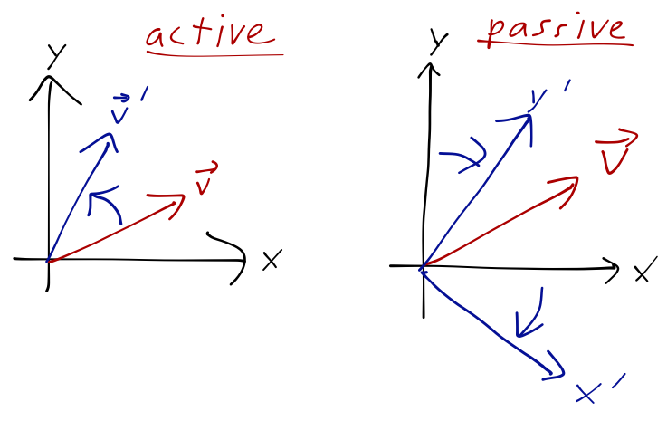
• Active View: We physically transform the state of the system, leaving our coordinate system and measurement devices fixed. The state vector $|\psi ⟩$ is mapped to a new vector $|{\psi }^{\prime }⟩=U(g)|\psi ⟩$. This is the standard perspective in quantum mechanics.
• Passive View: We consider the state vector $|\psi ⟩$ to be fixed, but we transform our description of it by changing the coordinate system (the basis vectors). This is equivalent to transforming the operators that represent observables.

Let's see how an observable, represented by a Hermitian operator $A$, transforms. The expectation value of $A$ in the transformed state $|{\psi }^{\prime }⟩$ must be equal to the expectation value of some transformed operator $A^{\prime }$ in the original state $|\psi ⟩$.

Substituting $|{\psi }^{\prime }⟩=U|\psi ⟩$ (we drop the $(g)$ for brevity):

Comparing the two expressions, we identify the transformation rule for operators:

This is the standard transformation law for an operator in the Heisenberg picture. A key consequence is that an operator $A$ is invariant under the symmetry $U$ if $A^{\prime }=A$, which implies $U^{†}AU=A$, or $[A,U]=0$. This direct link between symmetry and commutation is fundamental, and we will return to it in our next lesson.

2. Anti-Unitary Operators: The Case of Time Reversal

Wigner's theorem left open a second possibility: anti-unitary operators. While rarer, they are not a mere mathematical curiosity. They are essential for describing certain discrete symmetries, the most important of which is time reversal.

Let's denote the time-reversal operator by $\mathcal{T}$. Intuitively, we expect it to reverse the direction of motion. For a classical particle, this means its position is unchanged, but its momentum (and angular momentum) is inverted:

If $\mathcal{T}$ were a unitary operator in quantum mechanics, we would run into immediate contradictions. Consider the canonical commutation relation $[\hat{x},{\hat{p}}_x]=i\hslash$. Applying the unitary transformation rule:

But we also have:

This leads to the absurdity $-i\hslash =i\hslash$. The only way out is if the operator $\mathcal{T}$ is anti-linear, meaning it complex-conjugates any scalar it passes: $\mathcal{T}(i\hslash )=(i\hslash {)}^{\ast }\mathcal{T}=-i\hslash \mathcal{T}$. This resolves the contradiction.

A similar argument arises from the time-dependent Schrödinger equation, $i\hslash \frac{\partial }{\partial t}|\psi ⟩=H|\psi ⟩$. A time-reversal transformation involves taking $t\to -t$. For the equation to remain covariant (i.e., have the same form), the operator must also complex conjugate the equation to flip the sign of the $i$ on the left-hand side.

Formal Properties of Anti-Unitary Operators

This leads us to the formal definition. An operator $A$ is anti-linear if, for any vectors $|{\psi }_1⟩,|{\psi }_2⟩$ and complex scalars $c_1,c_2$:

An operator $\mathcal{T}$ is anti-unitary if it is anti-linear and also preserves the norm, which for anti-linear operators means:

This property ensures that transition probabilities $|⟨\varphi |\psi ⟩{|}^2$ are preserved, fulfilling the condition of Wigner's theorem.

The following resource provides a rigorous and clear treatment of these concepts. It defines anti-linear and anti-unitary operators, explains the difficulties they pose for the standard Dirac notation, and presents the key arguments for why time reversal must be anti-unitary.

3. Constructing the Time-Reversal Operator $\mathcal{T}$

Now that we understand the required properties of $\mathcal{T}$, how do we construct it for a given system? The form of $\mathcal{T}$ depends on the representation and the degrees of freedom (spatial and spin).

A general strategy is to decompose $\mathcal{T}$ into a product of a simple, universal anti-linear operator and a specific unitary operator: $\mathcal{T}=UK$.

• $K$ is the complex conjugation operator. Its definition depends on the basis. In the position basis, it simply takes the complex conjugate of the wavefunction: $K\psi (\mathbf{r})={\psi }^{\ast }(\mathbf{r})$.
• $U$ is a unitary operator, chosen to fix the transformation properties of observables like spin that are not correctly handled by $K$ alone.

System 1: Spinless Particle

For a particle without spin, the situation is simple. The time-reversal operator is just the complex conjugation operator in the position representation.

Let's check this. The position operator $\hat{\mathbf{r}}$ is real in this basis, so $\mathcal{T}\hat{\mathbf{r}}{\mathcal{T}}^{-1}=K\hat{\mathbf{r}}{K}^{-1}=\hat{\mathbf{r}}$. The momentum operator is $\hat{\mathbf{p}}=-i\hslash \nabla$.

This reproduces the required classical behavior.

This next video clip gives a concise derivation showing how $\mathcal{T}$ acts as complex conjugation on a wave function.

System 2: Particle with Spin

For a particle with spin, $K$ alone is not sufficient. Spin $\mathbf{S}$ is a form of angular momentum, so we require $\mathcal{T}\mathbf{S}{\mathcal{T}}^{-1}=-\mathbf{S}$. In the standard basis where $S_z$ is diagonal, the matrices for $S_x$ and $S_z$ are real, while $S_y$ is purely imaginary. The action of complex conjugation $K$ is:

• $K{S}_x{K}^{-1}=S_x^{\ast }=S_x$
• $K{S}_y{K}^{-1}=S_y^{\ast }=-S_y$
• $K{S}_z{K}^{-1}=S_z^{\ast }=S_z$

This is incorrect; we need to flip the signs of $S_x$ and $S_z$ as well. We can achieve this by applying an additional unitary transformation. The standard choice is a rotation by $\pi$ about the y-axis, $U=e^{-i\pi S_y/\hslash }$. This rotation flips $S_x$ and $S_z$ while leaving $S_y$ unchanged.
Combining the two operations, we get the full time-reversal operator for a system with spin:

For a spin-1/2 particle, $S_y=(\hslash /2){\sigma }_y$, and the unitary operator becomes $e^{-i(\pi /2){\sigma }_y}=-i{\sigma }_y$. So, for a two-component spinor wave function, the transformation is:

This construction is elegant and powerful. The following reading walks through the derivation in full detail, from the basic requirement $\mathcal{T}\mathbf{S}{\mathcal{T}}^{-1}=-\mathbf{S}$ to the final form for a multi-particle system.

Conclusion

In this lesson, we have put Wigner's theorem into practice. We established how to represent symmetry operations and how they act on the states and observables of a quantum system.

Key Takeaways:

• Symmetries associated with a group $G$ are realized as a unitary representation, a homomorphism from $G$ into the group of unitary operators $U(\mathcal{H})$.
• Unitary operators transform states via $|{\psi }^{\prime }⟩=U|\psi ⟩$ and operators via $A^{\prime }=U^{†}AU$.
• The time-reversal symmetry $\mathcal{T}$ requires an anti-unitary representation to be consistent with the fundamental laws of quantum mechanics.
• Anti-unitary operators are anti-linear and transform inner products as $⟨\mathcal{T}\varphi |\mathcal{T}\psi ⟩=⟨\varphi |\psi {⟩}^{\ast }$.
• The time-reversal operator $\mathcal{T}$ can be constructed as the product $\mathcal{T}=UK$, where $K$ is complex conjugation and $U=e^{-i\pi S_y/\hslash }$ is a spin-dependent rotation.

We now have a solid operational understanding of how to represent symmetries in quantum mechanics. In our next lesson, we will explore one of the most profound physical consequences of these representations: the connection between the symmetry group of a Hamiltonian and the degeneracy of its energy levels.