Space-Time Complexity Analysis

Understanding Space Complexity

While your work as a data scientist often involves powerful hardware, memory is never truly infinite. Inefficient memory usage can lead to slow performance or outright crashes, whether you're processing a terabyte-scale dataset on a distributed cluster or deploying a model on a memory-constrained device like a smartphone.

Space complexity measures the total amount of memory an algorithm requires to run, expressed as a function of the input size, $n$. Just like with time complexity, we use Big-O notation to describe its growth rate.

An algorithm's memory usage can be broken down into a few key parts.

To summarize the key points from your reading:

• Input Space: The memory used to store the input data itself. For an array of size $n$, this is $O(n)$.
• Auxiliary Space: The extra or temporary memory an algorithm uses during its execution. This includes variables, data structures, and any other allocated space.
• The Interview Standard: In coding interviews, when asked for "space complexity," the expectation is almost always to analyze the auxiliary space. You should generally assume the input space is a given and focus on the additional memory your algorithm requires. It's good practice to clarify this assumption with your interviewer: "Excluding the space for the input itself, the auxiliary space complexity is..."

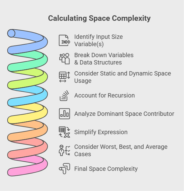
Calculating Space Complexity: From Constant to Linear

Let's analyze the space complexity of a few algorithms. The process is similar to analyzing time complexity: we identify what memory is being allocated and how its size relates to the input $n$.

The following video provides excellent visual examples of how to analyze space for a few common algorithms you've already seen.

Let's recap the common space complexity classes with Python examples:

• O(1) - Constant Space: The algorithm uses a fixed amount of memory regardless of the input size. This is the most space-efficient category.

  
  
  
  # Swaps two numbers in-place
  def swap(a, b):
  
  
  
      # Uses a fixed number of variables, regardless of the values of a and b.
      temp = a
      a = b
      b = temp
  
  
  
      # Auxiliary space: O(1)
  

• O(n) - Linear Space: The extra space required grows linearly with the input size. This often happens when you create a copy of the input or a new data structure of a similar size.

  
  
  
  # Creates a new list containing the doubled values of the input list.
  def double_values(numbers):
      doubled_list = [] # Initialize an empty list
      for num in numbers:
          doubled_list.append(num * 2)
      return doubled_list
  
  
  
      # Auxiliary space: O(n), where n is len(numbers), for storing doubled_list.
  

• O(log n) - Logarithmic Space: The space grows logarithmically with the input. As seen in the video, this is typical for the recursion stack in well-balanced divide-and-conquer algorithms. The recursive implementation of binary search is a classic example.

• O(n²) - Quadratic Space: The space grows with the square of the input size. A common example is creating an adjacency matrix to represent a graph with $n$ vertices.

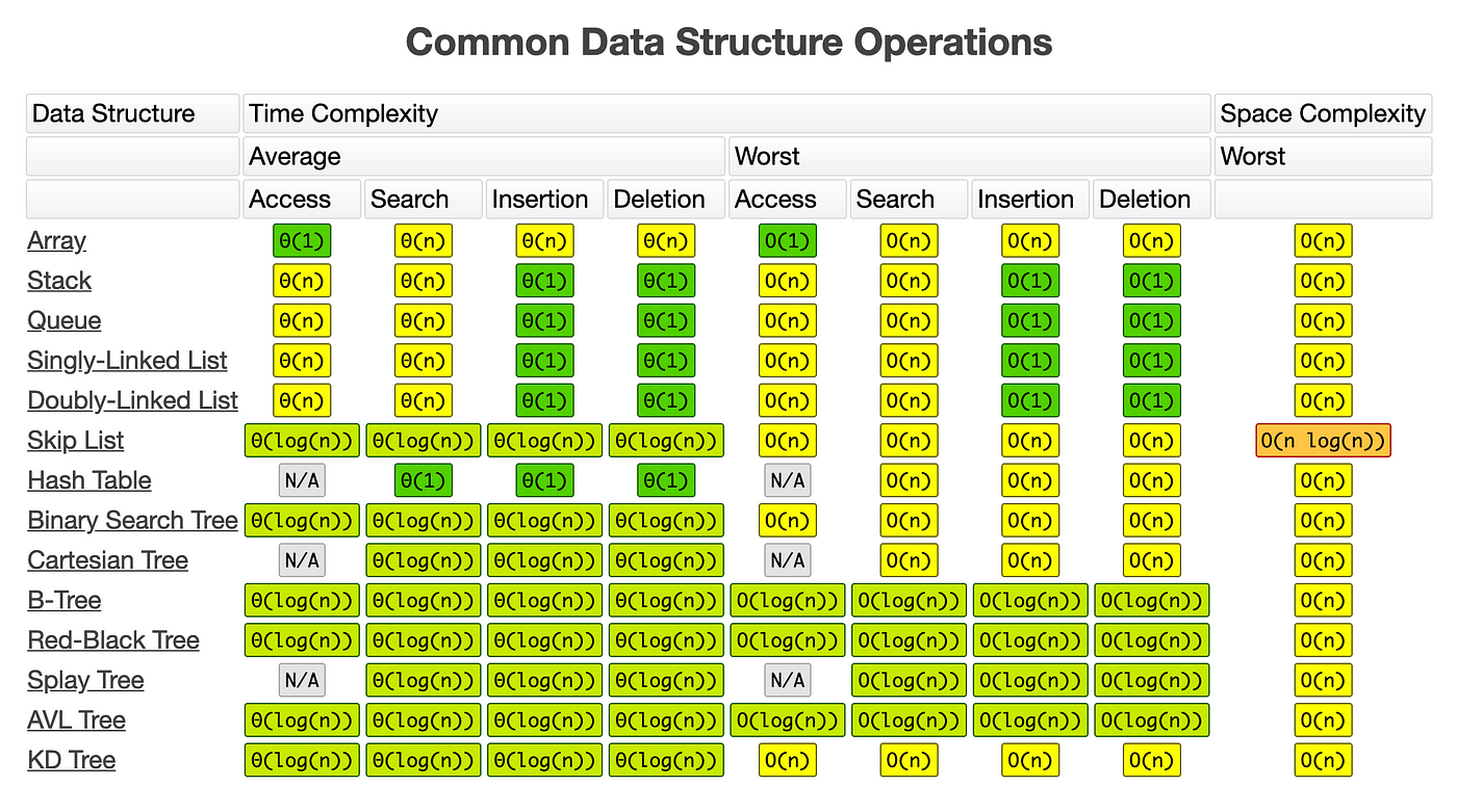
The Time-Space Trade-off

Now we arrive at one of the most important practical concepts in algorithm design: the time-space trade-off. It's rare to find an algorithm that is optimal in both time and space. More often, you'll face a choice:

• Use more memory to make the algorithm run faster.
• Save memory at the cost of a slower runtime.

This trade-off is at the heart of countless interview problems. Recognizing when you can "buy" a faster runtime with extra space is a key skill. The HashMap (or dict in Python) is the quintessential tool for this trade.

Let's consider another example you may be familiar with from your ML work: memoization. Think of calculating the n-th Fibonacci number.

1. Naive Recursive Solution:

   • Time: $O(2^n)$. Terribly slow because it re-computes the same values over and over.
   • Space: $O(n)$. The space is determined by the maximum depth of the recursion stack.

2. Memoized (Top-Down DP) Solution:

   • Time: $O(n)$. Each Fibonacci number is computed only once.
   • Space: $O(n)$. We use $O(n)$ space for the recursion stack plus $O(n)$ space for the memoization cache (e.g., a dictionary or array). The total is still $O(n)$.

Here, we've invested $O(n)$ auxiliary space for the cache and, in doing so, dramatically reduced the time complexity from exponential to linear. This is a powerful demonstration of the time-space trade-off.

Conclusion

In this lesson, we've completed our foundational understanding of algorithm analysis by adding space complexity to your toolkit. You are now equipped to analyze both the time and memory requirements of an algorithm—a comprehensive skill set required for any technical interview.

Key Takeaways:

• Space Complexity measures an algorithm's memory usage as a function of its input size, typically focusing on auxiliary space.
• Memory usage comes from variables, data structures, and the recursion call stack.
• The same Big-O notation is used to classify space complexity, with O(1) (constant), O(n) (linear), and O(log n) (logarithmic) being the most common.
• The Time-Space Trade-off is a fundamental concept: you can often achieve faster runtimes by using more memory, or vice-versa. Using a dict (HashMap) to cache results or seen values is the classic example of this trade-off.

As you move forward, make it a habit to analyze both time and space complexity for every problem you solve. In an interview, being able to articulate the trade-offs of your chosen approach demonstrates a deeper level of understanding.

In our next lesson, we will begin our dive into concrete data structures, starting with dynamic arrays (what you know as lists in Python). We will analyze the time and space complexity of their core operations and see how these theoretical concepts apply in practice.