Big-O Algorithm Analysis

Introduction

Welcome to the start of your journey to master Data Structures and Algorithms. As we discussed, building a rock-solid foundation in DSA is the first critical step for the top-tier data science and machine learning roles you're targeting. This first lesson tackles the most fundamental concept in algorithm analysis: time complexity.

The goal of this lesson is to enable you to analyze an algorithm's efficiency using Big-O notation. This is the universal language for discussing performance in technical interviews. We will explore what time complexity represents, why it's crucial even with modern hardware, and how to calculate it for various code structures. By the end of our session, you will be able to look at a piece of code and confidently describe how its runtime scales with the size of its input.

Why Time Complexity Matters

You might wonder if optimizing algorithms is still necessary given the immense power of today's computers, especially in the ML world where massive computational resources are common. The answer is an emphatic yes. An inefficient algorithm can bring even the most powerful hardware to its knees when faced with large-scale data.

To build an intuition for this, let's start with a memorable story that illustrates the core idea of scalability.

Big O Notation

The video "Big O Notation" from HackerRank, presented by Gayle Laakmann McDowell (author of Cracking the Coding Interview), uses a fantastic real-world analogy to contrast an algorithm that scales with its input size versus one that doesn't.

Please watch the introduction, from the beginning up to the end of the pigeon-versus-internet story. As you watch, consider how the "pigeon" method's time is independent of the data size, while the "internet" method's time is directly proportional to it.

As the video explains, the pigeon's delivery time is constant, regardless of how much data is on the USB stick. We call this $O (1)$ . The internet transfer time, however, grows linearly with the amount of data; twice the data takes roughly twice the time. We call this $O (n)$ .

This is the essence of time complexity analysis: we are not measuring the exact runtime in seconds, but rather describing how the number of operations an algorithm performs grows as the input size, $n$ , increases. This allows us to compare algorithms in a way that is independent of the programming language, hardware, or specific input values.

The Rules of Big-O Notation

To analyze time complexity, we count the number of "basic instructions" an algorithm executes. These are simple operations like arithmetic, comparisons, or variable assignments. Big-O notation gives us a high-level way to express this count by focusing on the "big picture" of how the count grows. This is achieved by applying a few simple rules.

Big O Notation

The same HackerRank video provides a concise explanation of the four essential rules for simplifying complexity expressions into Big-O notation.

Watch the segment that covers the four rules of Big-O. Focus on understanding each principle: Add Runtimes: For sequential, independent steps. Drop Constants: O(2n) is simplified to O(n). Different Inputs, Different Variables: Use O(a \cdot b) for nested loops over two different arrays of lengths a and b. Drop Non-Dominant Terms: O(n^2 + n) is simplified to O(n^2).

Let's quickly formalize this. If we meticulously count the operations in an algorithm and arrive at a function like $f (n) = 3 n^{2} + 50 n + 100$ , we apply the rules to find the Big-O complexity:

Identify the dominant term: As $n$ gets very large, the $3 n^{2}$ term will grow much faster and contribute far more to the total value than $50 n$ or $100$ . So, $n^{2}$ is the dominant part. We drop the non-dominant terms: $3 n^{2}$ .
Drop the constant coefficient: The constant multiplier 3 doesn't change the fundamental quadratic growth rate. Whether it's $3 n^{2}$ or $10 n^{2}$ , the shape of the growth curve is the same. So we drop the 3.

The final time complexity is $O (n^{2})$ . This simplification is powerful because it tells us the fundamental scaling nature of the algorithm: if we double the input size, the runtime will roughly quadruple.

A Tour of Common Complexities

In coding interviews, you'll repeatedly encounter a handful of common complexity classes. Recognizing the patterns of code that lead to each one is a vital skill.

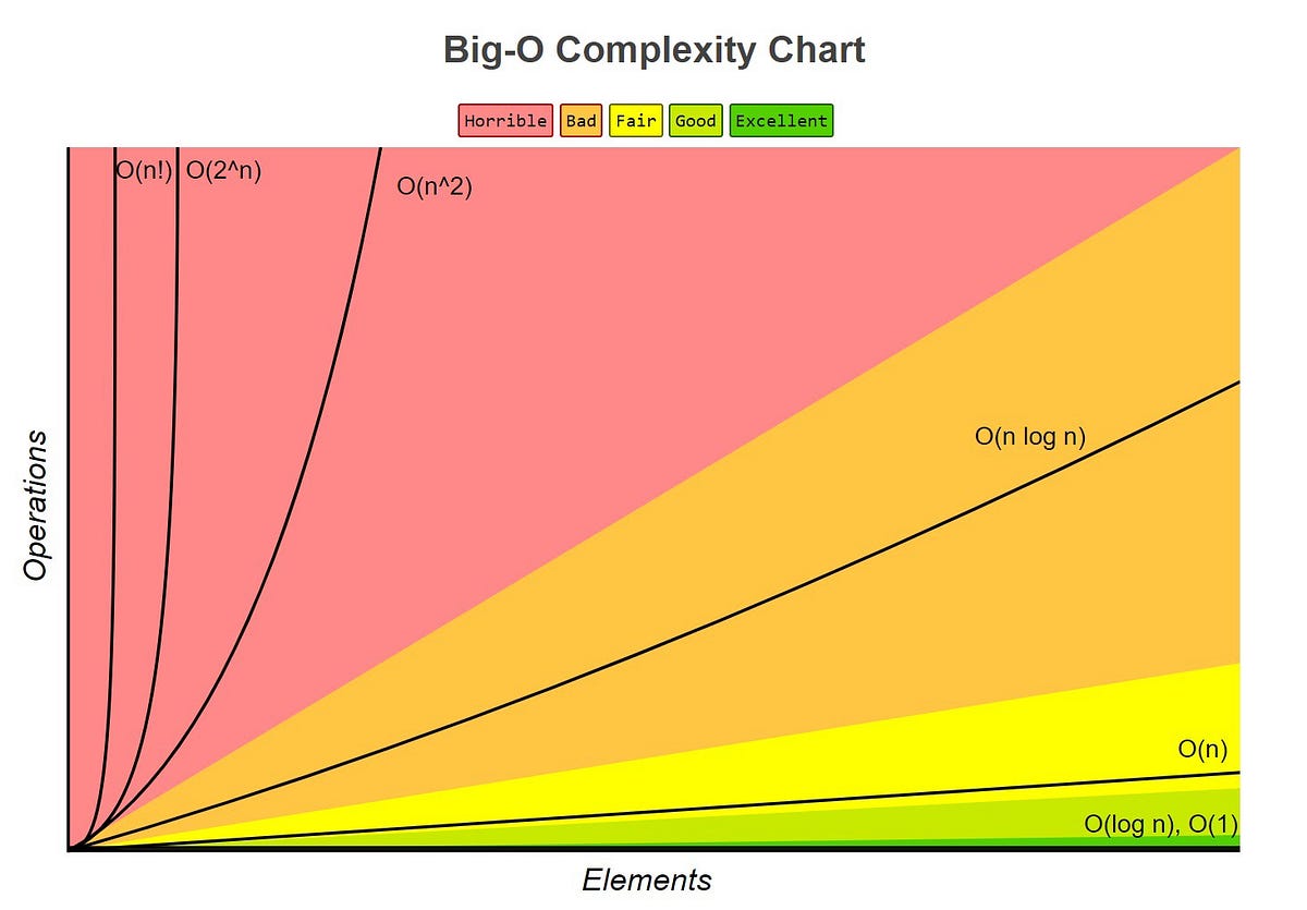
This chart illustrates the growth rates of common time complexities. As you can see, the difference between "Good" and "Horrible" performance becomes dramatic as the number of elements increases.

The following video provides an excellent, practical overview of these complexity classes with code examples that you are likely to see in interview problems.

Big-O Notation - For Coding Interviews

The "Big-O Notation - For Coding Interviews" video from the popular channel NeetCode is tailored specifically for interview preparation. It connects abstract complexities to concrete algorithm types.

Watch the following segments, paying close attention to the code patterns and algorithm examples associated with each complexity: Constant Time: O(1) Linear Time: O(n) Logarithmic Time: O(log n) Linearithmic Time: O(n log n) Quadratic Time: O(n^2) Exponential Time: O(2^n)

To help you consolidate this information, here is a quick-reference table summarizing the key complexities and their common Python examples.

A summary of common Big-O notations, their meanings, and corresponding Python examples you'll encounter frequently.

Worst-Case Analysis: The Interview Standard

An algorithm's runtime can sometimes depend on the specific values in the input, not just its size. For example, when searching for an element in an array, we might find it at the very first position (best case) or the very last (worst case).

So which one do we care about? In algorithm analysis, and especially in coding interviews, we are almost always concerned with the worst-case time complexity.

Big O Notation and Time Complexity Guide: Intuition ...

The DataCamp article "Big O Notation and Time Complexity Guide" provides a clear rationale for this focus on the worst case.

Please read the section Worst Case and Best Case. The three points listed there summarize why this perspective is the most practical and reliable for designing robust systems.

Focusing on the worst-case scenario provides a performance guarantee. When you state that an algorithm is $O (n^{2})$ , you are communicating that its performance will never be worse than this quadratic scaling, which is crucial for predicting system behavior under heavy load.

Conclusion

In this introductory lesson, we have laid the essential groundwork for analyzing algorithm efficiency.

Key Takeaways:

Time complexity describes how an algorithm's runtime scales with its input size, $n$ .
Big-O notation is a high-level measure of this growth rate, focusing on the dominant term and ignoring constants.
The most common complexities range from the highly efficient $O (1)$ and $O (lo g n)$ to the extremely slow $O (n^{2})$ and $O (2^{n})$ .
Recognizing code patterns like loops, nested loops, and recursive calls is key to identifying the complexity.
For interviews and robust system design, we almost always analyze the worst-case time complexity.

Mastering this concept is non-negotiable for success in technical interviews. As you work through problems, make it a habit to consciously analyze the time complexity of every solution you devise.

In our next lesson, we will introduce the other side of the coin: space complexity. We'll explore how to analyze an algorithm's memory usage and discuss the critical trade-offs that often exist between time and space efficiency.