Welcome to the next stage of our journey into GPU architecture. In our last lesson, we charted the GPU's memory hierarchy, creating a qualitative map of the trade-offs between speed, size, and proximity to the compute units. We saw that the entire architecture, particularly the SIMT model, is designed to hide the high latency of off-chip memory by maximizing throughput.
Today, we transition from this qualitative map to a quantitative one. Our goal is to establish the theoretical "performance budget" of a GPU. We will learn how to calculate the two most important numbers that define a hardware's performance envelope: its peak computational throughput, measured in Floating Point Operations Per Second (FLOP/s), and its peak memory bandwidth, measured in Gigabytes per second (GB/s). These two figures represent the "speed of light" for a given GPU—the absolute ceiling on performance. Understanding this budget is the first step for any serious performance engineer; it's the benchmark against which we will measure all our future optimization efforts for GPT-2 and ResNet-50.
Calculating Peak Compute Throughput (FLOP/s)
The first pillar of our performance budget is raw computational power. For scientific and deep learning workloads, this is measured by how many floating-point operations the chip can execute per second.
The general formula to calculate this peak performance is a product of the chip's key characteristics:
The most nuanced part of this calculation is the "FLOP/s per SM" term, as it depends heavily on the data type (e.g., FP32, FP16, BF16) and the specific compute units being used. On modern GPUs, the highest throughput for deep learning tasks is achieved not by the general-purpose CUDA cores, but by specialized hardware called Tensor Cores.
The following blog post provides an excellent guide on how to perform this calculation for a modern GPU like the NVIDIA H100.
Inside NVIDIA GPUs: Anatomy of high performance matmul kernels
This post by Aleksa Gordić dives into the specifics of GPU performance. We'll use it to get the formula for calculating the theoretical peak throughput.
Please read the section titled Speed of light and power throttling. Pay close attention to the formula perf = freq_clk_max * num_tc * flop_per_tc_per_clk. The accompanying figure provides a concrete derivation for BF16 performance on an H100, which we will replicate.
Let's use the information from the reading and other public specifications to perform these calculations for our target GPU, the NVIDIA H100 (SXM5 variant).
H100 Peak Throughput: A Worked Example
We'll calculate the peak performance for three key data types: standard single-precision (FP32), and the two dominant mixed-precision formats, Bfloat16 (BF16) and FP16.
1. H100 Hardware Specifications:
From the "Stanford Seminar" video and the "Inside NVIDIA GPUs" article, we can gather these key specifications for the H100 SXM5:
- Max Clock Frequency: ~1.98 GHz
- Streaming Multiprocessors (SMs): 132
- Tensor Cores per SM: 4 (4th Generation)
- FP32 CUDA Cores per SM: 128
2. FP32 Peak Performance (using CUDA Cores):
Each of the 128 FP32 cores in an SM can execute a Fused Multiply-Add (FMA) operation per clock cycle. An FMA (a*b + c) counts as 2 FLOPs (one multiplication, one addition).
- FLOP/s per SM = 128 cores × 2 FLOPs/core/clock = 256 FLOPs/SM/clock
- Total Peak FP32 FLOP/s =
3. BF16/FP16 Peak Performance (using Tensor Cores):
This is where things get interesting. Tensor Cores are specialized circuits that perform matrix-matrix operations at incredible speeds. The 4th generation Tensor Cores in the H100 are exceptionally powerful. As per the "Inside NVIDIA GPUs" article, each of the 4 Tensor Cores per SM can perform 512 BF16 FLOPs per clock cycle for dense operations.
- BF16 FLOP/s per SM = 4 TCs/SM × 512 FLOPs/TC/clock = 2048 FLOPs/SM/clock
- Total Peak BF16 FLOP/s =
Notice the staggering difference: the H100 offers nearly 8 times more throughput for BF16/FP16 operations on its Tensor Cores than for FP32 operations on its CUDA cores. This is the hardware incentive behind mixed-precision training.
Furthermore, modern GPUs support structured sparsity, a feature where the hardware can ignore zero-valued weights in a 2:4 sparse matrix pattern to double the throughput. With sparsity enabled, the peak BF16/FP16 performance doubles to over 1000 TFLOP/s (1 PetaFLOP/s).
This dramatic increase in throughput from using specialized data formats and hardware units is a core theme in modern GPU design.
Stanford Seminar - Nvidia’s H100 GPU
The Stanford seminar on the H100 provides a summary chart that visualizes these compounding gains.
Watch the segment from this chart that breaks down the 6x throughput increase from the A100 to the H100. Notice how the gains come from multiple factors: more SMs, a new Tensor Core generation, new data formats (FP8), and higher clock frequency.
Calculating Peak Memory Bandwidth (HBM)
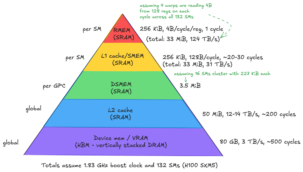
The second pillar of our performance budget is memory bandwidth. No matter how fast your compute units are, they are useless if you cannot feed them data. The primary bottleneck for data delivery is the bandwidth between the GPU chip and its main memory (HBM).
Unlike FLOP/s, you don't typically calculate peak HBM bandwidth from first principles (like memory clock and bus width). It's a headline specification provided by the manufacturer. Our job is to find and understand this number.
Stanford Seminar - Nvidia’s H100 GPU
Let's return to the Stanford seminar, where the speaker explicitly states the HBM bandwidth for the H100.
Watch the clip from "Hopper has five hbm3 sites". This section gives the total memory capacity (80 GB) and the crucial peak memory bandwidth figure.
As the video confirms, the NVIDIA H100 SXM5 GPU has a peak memory bandwidth of 3 Terabytes per second (TB/s). This is an immense number, far exceeding the memory bandwidth of even the most advanced CPU systems (which are typically in the range of 100-200 GB/s). This is why GPUs excel at problems that involve processing large amounts of data in parallel.
The Hardware Performance Budget and Arithmetic Intensity
We have now established the two pillars of our H100 performance budget:
- Peak Compute (BF16 Dense): ~535 TFLOP/s
- Peak Memory Bandwidth: 3 TB/s
These two numbers are not independent; their ratio defines a critical characteristic of the hardware itself. This brings us to the concept of Arithmetic Intensity (AI).
Arithmetic Intensity is the ratio of floating-point operations performed to the bytes of data moved from main memory to serve those operations.
A high AI means you are doing a lot of computation for every byte you fetch, while a low AI means your computation is "light" and you are spending most of your time waiting for data.
We can use our two peak performance numbers to calculate the ridge point, which is the minimum AI a workload must have to be theoretically capable of being limited by compute rather than memory bandwidth.
For our H100 (using BF16):
This number is fundamental. It tells us that any kernel or algorithm running on this H100 with an arithmetic intensity less than 178 FLOPs/Byte will be memory-bound. Its performance will be limited by the 3 TB/s HBM bandwidth, and the powerful Tensor Cores will be starved for data, sitting idle. Conversely, any workload with an AI greater than 178 FLOPs/Byte has the potential to be compute-bound, limited by the 535 TFLOP/s compute ceiling.
This concept is visually captured by the Roofline Model, which we will explore in depth in our next lesson.
Conclusion
In this lesson, we have armed ourselves with the essential tools to quantify a GPU's performance potential. We've moved beyond a simple architectural diagram to a concrete performance budget, grounded in numbers.
Key Takeaways:
- Peak FLOP/s is calculated based on clock speed, SM count, and the throughput of the specific compute units (CUDA cores or Tensor Cores) for a given data precision.
- Tensor Cores provide a massive boost in throughput for mixed-precision formats (BF16, FP16, FP8), creating a strong hardware incentive for their use in deep learning.
- Peak HBM Bandwidth is a critical, top-line specification that determines how quickly the GPU can be fed data from its main memory. For an H100, this is 3 TB/s.
- The ratio of peak FLOP/s to peak bandwidth gives the machine's Arithmetic Intensity ridge point, a crucial value that determines whether a workload will be memory-bound or compute-bound. For an H100, this is approximately 178 FLOPs/Byte for BF16 workloads.
We have now defined the "roof" of our performance model. In our next lesson, we will put this budget to use. We will estimate the FLOPs and memory requirements of our case study models, GPT-2 small and ResNet-50. By calculating their arithmetic intensity, we will use the Roofline Model to predict whether their key layers are fundamentally limited by compute or memory, setting the stage for all future optimization work.