Hello! In our previous lesson, we explored the GPU's dynamic execution model, SIMT, and saw how the hardware uses massive threading and warp scheduling to "hide" the latency of memory operations. This naturally leads to the question: what is this latency we are trying so hard to hide?
This lesson dives deep into that question by charting the GPU's memory landscape. We will diagram the complete memory hierarchy, from the registers sitting right next to the execution units to the high-capacity DRAM on the package. Our goal is to map out each level, understanding its physical location, logical scope, and—most importantly—its characteristic size, latency, and bandwidth. For a systems engineer, this map is not just an architectural curiosity; it is the fundamental schematic for optimizing performance. Every performant kernel is, at its core, an exercise in intelligent data placement within this hierarchy.
The Memory Wall and the GPU's Philosophy
The central challenge in modern computing is often called the "Memory Wall": computational power has grown much faster than the ability of memory systems to supply data. As a deep learning practitioner, you've implicitly dealt with this every time you've been bottlenecked by data loading rather than model computation.
GPUs and CPUs attack this problem from different philosophical standpoints, a theme we touched on in our first lesson.
- CPUs are latency-oriented. They use large, multi-level caches and complex logic to reduce the time a single thread has to wait for data.
- GPUs are throughput-oriented. They accept that high latency to main memory is a fact of life. Instead of trying to eliminate it for a single thread, they use the SIMT model and massive parallelism to ensure that some work is always being done, hiding latency by switching to other ready warps.
The following reading provides an excellent introduction to this concept and establishes the two crucial lenses through which we must view GPU memory: its physical location (where the bits are stored) and its logical scope (which threads can access it).
This article from the Uplatz blog provides a comprehensive, expert-level analysis of the CUDA memory hierarchy. It perfectly frames the problem as one of data flow orchestration.
Please read the introduction and the first section, "Architectural Foundations". Pay close attention to the distinction between the GPU's throughput-oriented design and the critical concept of separating Physical Location from Logical Scope. The discussion of "Local Memory" is a prime example of why this is so important.
A Tour of the Memory Hierarchy
The GPU memory system is a pyramid. At the top, you have tiny, incredibly fast memory resources private to a single thread. As you descend the pyramid, the memory capacity grows enormously, but access latency increases and bandwidth decreases dramatically. Let's walk through this hierarchy, starting from the execution units and moving outwards.
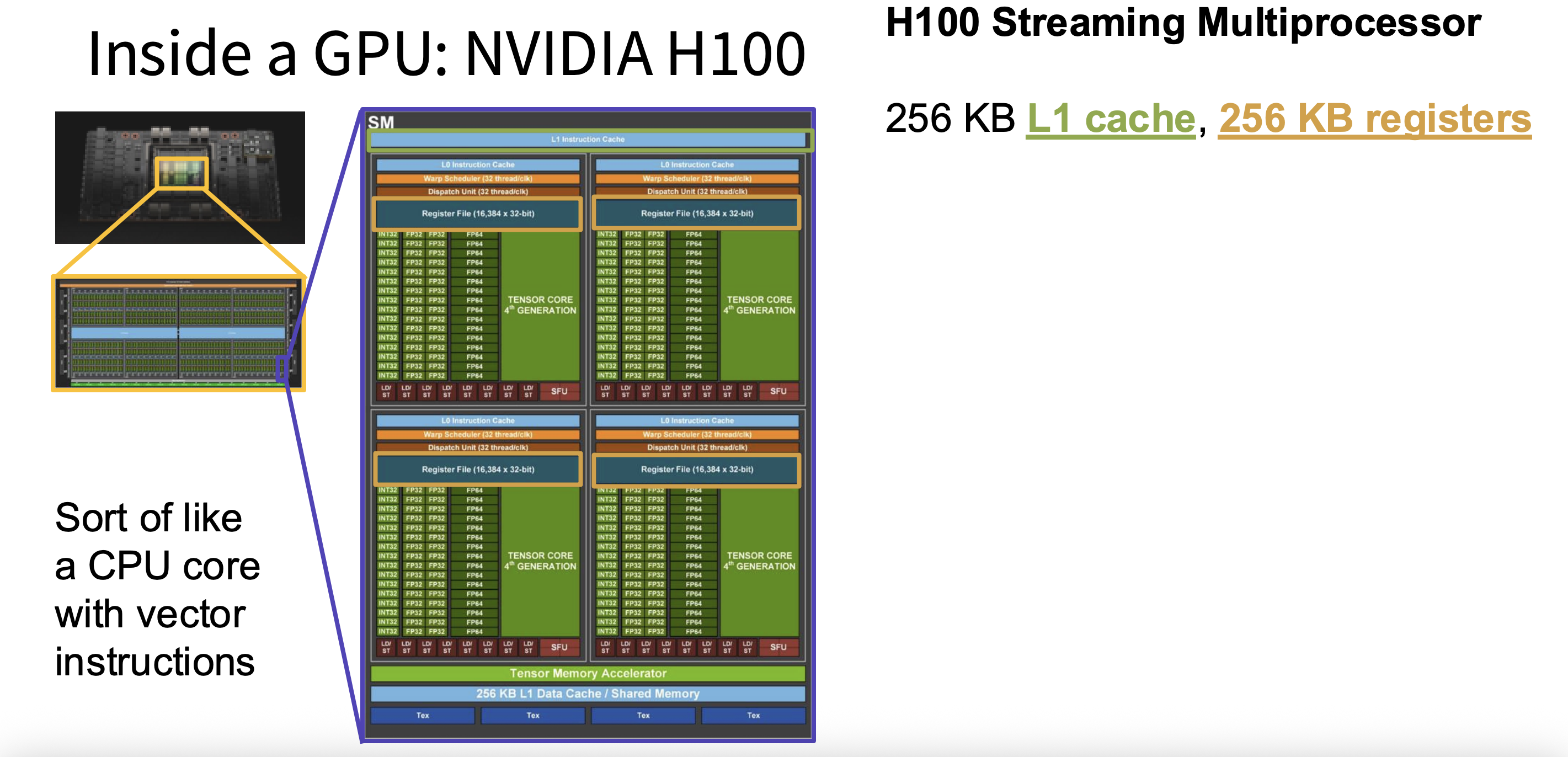
A modern NVIDIA H100 GPU provides a concrete example of this structure. The following diagram shows a single Streaming Multiprocessor (SM) and its local memory components.
1. Registers
- Physical Location & Scope: The register file is a bank of memory located directly on the SM, as seen in the diagram above. Registers are the fastest memory on the GPU, private to a single thread.
- Characteristics:
- Latency: Effectively zero (~1 clock cycle). Access is part of the instruction execution itself.
- Bandwidth: Massive. The aggregate bandwidth across all SMs is on the order of tens of TB/s.
- Size: The total register file per SM is large (e.g., 256 KB on H100), but this finite resource must be divided among all threads resident on the SM. An H100 thread can use up to 255 registers.
- The Catch (Occupancy): Register usage is a primary constraint on occupancy. If your kernel uses many registers per thread, fewer threads (and thus fewer warps) can be active on the SM at once. This reduces the SM's pool of ready warps, diminishing its ability to hide memory latency. We will explore this trade-off in detail later.
2. L1 Cache / Shared Memory
As the H100 Streaming Multiprocessor image shows, each SM contains a block of fast on-chip SRAM that serves a dual purpose.
- Physical Location & Scope: This memory is on the SM. It is logically partitioned into two distinct spaces:
- L1 Data Cache: A hardware-managed cache for global and local memory accesses. It's transparent to the programmer and works to reduce latency for frequently accessed off-chip data.
- Shared Memory: A programmer-managed "scratchpad" memory. Its scope is a thread block. All threads within a single block can use it to share data and cooperate. This makes it an incredibly powerful tool for optimization.
- Characteristics:
- Latency: Very low, on the order of 20-50 clock cycles. It's slightly slower than registers but dramatically faster than off-chip memory.
- Bandwidth: Extremely high, comparable to registers. The aggregate bandwidth is in the tens of TB/s range.
- Size: The total size of this unified block on an H100 SM is 256 KB. CUDA allows the programmer to express a preference for how much of this is dedicated to shared memory versus L1 cache.
This video from a Stanford seminar on the H100 provides a high-level overview of the memory hierarchy, confirming the sizes of these on-SM resources.
Stanford Seminar - Nvidia’s H100 GPU
This Stanford seminar provides insights directly from NVIDIA architects on the H100 GPU.
First, watch the brief segment from the description of the SM, which states the 256 KB size of the unified L1/Shared Memory. Then, jump to the section on data locality, which maps the CUDA programming concepts of grids, blocks, and threads to the hardware hierarchy of L2/HBM, SM-localized storage (L1/Shared), and the register file.
3. L2 Cache
- Physical Location & Scope: The L2 cache is a large pool of SRAM on the GPU chip itself, but it is not part of any single SM. It is shared by all SMs and acts as a unified, last-level cache before accessing main memory.
- Characteristics:
- Latency: Mid-range, around 200 cycles. It's slower than L1 but serves as a crucial backstop.
- Bandwidth: High, in the range of 3-6 TB/s on an H100.
- Size: Large enough to be very effective. The H100 features a 50 MB L2 cache.
The following deep-dive analysis provides precise latency and bandwidth figures for the H100's cache system.
Nvidia's H100: Funny L2, and Tons of Bandwidth - Chips and Cheese
This article from "Chips and Cheese" is a detailed, quantitative analysis of the H100 memory subsystem based on microbenchmarks. It provides specific numbers that bring the abstract hierarchy to life.
First, read the section on L1, titled "Cache and Memory Setup". It confirms the size and low latency of the L1/Shared Memory block. Then, read the subsequent section on the L2 cache, starting from the discussion of L2, which details its size and the interesting non-uniform latency characteristic of its "near" and "far" partitions.
4. Global Memory (HBM)
This is the workhorse memory of the GPU, what is commonly referred to as VRAM.
- Physical Location & Scope: This is off-chip DRAM (Dynamic Random-Access Memory) that resides on the same physical package as the GPU die. Data center GPUs like the H100 use a technology called High-Bandwidth Memory (HBM), which involves stacking DRAM dies vertically to achieve an extremely wide memory interface. It is accessible by all threads in the grid and by the host CPU.
- Characteristics:
- Latency: High, in the range of 400-800 clock cycles. This is the latency that the GPU's architecture is built to hide.
- Bandwidth: While the "slowest" tier, its absolute bandwidth is immense, far exceeding what's available on CPU systems. An H100 provides up to 3 TB/s of HBM bandwidth. This is the headline memory bandwidth number for the GPU.
- Size: Very large, typically 80 GB for an H100.
This focus on maximizing bandwidth, even at the cost of higher latency, is a core tenet of GPU design for deep learning.
Stanford Seminar - Nvidia’s H100 GPU
Returning to the Stanford seminar, the speaker explains the design philosophy behind HBM.
Watch the section from "Hopper has five hbm3 sites" to understand the scale of HBM bandwidth. Then, watch the Q&A segment from "another question if you could" where the speaker explicitly states that for GPU workloads, bandwidth is prioritized over latency.
Clarifying Special Memory Spaces
The CUDA programming model exposes a few other memory spaces that are important to understand. They are not new physical memories but rather specialized access paths to the hierarchy we've just described.
- Local Memory: This is the most confusingly named space. It is logically private to a thread, but physically located in slow, off-chip Global Memory. The compiler uses Local Memory when a thread's private data is too large to fit in registers (a situation called "register spilling"). Accesses to local memory are slow and should be avoided.
- Constant Memory: A 64 KB read-only region of global memory that is cached in a dedicated on-chip constant cache. It is highly optimized for the access pattern where all 32 threads in a warp read from the exact same memory address. This results in a single read that is broadcast to all threads.
- Texture Memory: A read-only cache path optimized for spatial locality. It uses hardware from the GPU's graphics heritage to accelerate 2D and 3D memory access patterns, common in image processing and scientific simulations.
Synthesis: A Comparative Table
To bring everything together, we can summarize the hierarchy in a table. The latency and bandwidth numbers are approximate for a modern architecture like the H100 and serve to illustrate the orders of magnitude difference between the levels.
The Uplatz blog article provides an excellent summary table that we can use as a reference.
Please review the table in Section 8. It synthesizes the scope, location, and performance characteristics of each memory type.
Here is a condensed version of that information:
| Memory Type | Scope | Physical Location | Latency (Cycles) | Bandwidth (Aggregate) |
|---|---|---|---|---|
| Register | Thread | On-Chip (SM) | ~1 | ~20+ TB/s |
| Shared | Block | On-Chip (SM) | ~30-50 | ~19 TB/s |
| L1 Cache | (Hardware) | On-Chip (SM) | ~30-50 | High |
| L2 Cache | Device (Grid) | On-Chip (Shared) | ~200 | ~6 TB/s |
| Global (HBM) | Device (Grid) | Off-Chip DRAM | 400-800 | ~3 TB/s |
| Local | Thread | Off-Chip DRAM | 400-800 | ~3 TB/s |
Conclusion
In this lesson, we have constructed a detailed map of the GPU's memory hierarchy. We have seen how memory resources are stratified by their physical location, leading to a dramatic trade-off between capacity, latency, and bandwidth.
Key Takeaways:
- The GPU memory hierarchy is a pyramid: Registers at the peak are fastest but smallest, while Global Memory (HBM) at the base is largest but slowest.
- On-Chip Memory (Registers, Shared/L1, L2): Characterized by very low latency and extremely high bandwidth. The key to performance is maximizing the use of these resources to keep data close to the execution units.
- Off-Chip Memory (Global/HBM): Characterized by high latency and (relatively) lower bandwidth. The entire SIMT execution model is designed to hide this latency.
- Scope vs. Location: It is crucial to distinguish a memory space's logical scope (e.g.,
localto a thread) from its physical location (e.g.,off-chipDRAM). - Data Placement is Key: Writing efficient GPU kernels is fundamentally an algorithm of data movement: staging the right data in the right memory at the right time.
Now that we have a map of the memory system and its performance characteristics, our next step is to quantify the GPU's theoretical limits. In the upcoming lesson, we will learn how to compute the peak floating-point operations per second (FLOPs) and the peak memory bandwidth for a target GPU like the H100. These two numbers will form the "performance budget" we have to work with, setting the stage for analyzing and optimizing our case study models.