Optimizing PCIe Bandwidth for Model Training

The Host-Device Interconnect: A Bandwidth Choke Point

Before the GPU can perform any computation, it needs data—input batches, model weights, and more. This data originates in the host's main memory (RAM) and must travel to the GPU's high-bandwidth memory (HBM) over the PCIe bus. As the CUDA C++ Best Practices Guide emphasizes, this transfer is a costly operation that should be minimized.

The performance of this connection is defined by the PCIe standard's version and the number of "lanes" used. Each revision of the standard (e.g., 3.0, 4.0, 5.0) doubles the per-lane transfer rate, and a typical GPU uses an x16 (16-lane) connection for maximum throughput.

Let's calculate the theoretical bandwidth for a modern PCIe 4.0 x16 link, common in servers with A100 or H100 GPUs.

• Transfer Rate: 16 GT/s (Gigatransfers per second)
• Encoding: 128b/130b (128 data bits for every 130 bits transmitted)
• Per-Lane Throughput: $16\text{ Gb/s}\times \frac{128}{130}\approx 15.754\text{ Gb/s}$
• Converting to Bytes/s: $15.754\text{ Gb/s}/8\approx 1.969\text{ GB/s}$
• Total Bandwidth (x16): $1.969\text{ GB/s}\times 16\approx \text{31.5 GB/s}$

Compare this to the H100's HBM bandwidth of 3.35 TB/s. The connection to the host is over 100 times slower than the GPU's internal memory access. This stark difference underscores why minimizing host-device traffic is paramount.

From Theoretical to Effective Bandwidth

Just as with FLOPs, the theoretical bandwidth is a ceiling that is rarely achieved in practice. The actual measured rate is called effective bandwidth.

The CUDA Best Practices Guide provides a simple formula for its calculation:

For a round trip (e.g., copy from host to device and back), this would be:

One of the largest factors impacting effective bandwidth is the type of host memory used for the transfer.

Pageable vs. Pinned Memory

By default, memory allocated on the CPU is pageable, meaning the operating system can move its physical location in RAM (virtual memory management). However, for a high-speed Direct Memory Access (DMA) transfer, the GPU's copy engine needs a stable, physical memory address.

When you request a transfer from pageable memory, the CUDA driver must first copy the data into a temporary, non-pageable block of pinned memory before initiating the DMA transfer to the GPU. This staging copy introduces significant overhead and effectively halves the achievable bandwidth.

To get the best performance, you must allocate host-side buffers directly as pinned memory. This allows the GPU's copy engine to access the data directly without the intermediate copy.

As the video demonstrates, using pinned memory can nearly double the effective bandwidth of host-device transfers, bringing it much closer to the theoretical peak of the PCIe link. PyTorch's DataLoader exposes a pin_memory=True argument that handles this for you automatically for input data pipelines.

Estimating the Transfer Cost of a Training Step

Now, let's quantify the "cost" of these transfers by estimating the data movement in a single training step. The primary data transfers are:

1. Input Data: The batch of training data (e.g., text tokens, images) must be moved from host RAM to GPU HBM. Host -> Device.
2. Model State: This depends heavily on the training strategy. In a simple single-GPU setup, the model parameters, gradients, and optimizer states might all reside on the GPU, minimizing PCIe traffic. However, for large models that don't fit in GPU memory, a common technique is to offload parts of the model state to host RAM. This is a core feature of optimizers like DeepSpeed's ZeRO.

Let's analyze the cost of CPU offloading for the optimizer states and parameter updates. The image below illustrates a timeline for a single training step using ZeRO-Offload.

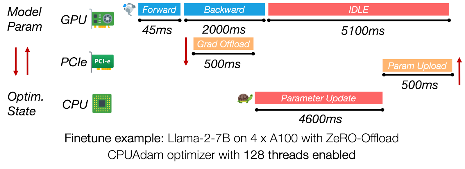
This timeline clearly shows the cost of offloading:

1. After the backward pass, gradients are computed on the GPU. They are then offloaded to the CPU (Grad Offload).
2. The CPU uses these gradients to perform the parameter update (the Adam optimizer is often faster on a multi-core CPU than on a GPU for this task).
3. The updated parameters are then uploaded back to the GPU (Param Upload) for the next forward pass.

Let's calculate this cost for our GPT-2 small (124M parameters) model, assuming mixed-precision training where the optimizer maintains an FP32 copy of the weights.

• Parameter/Gradient Size: A single FP32 value is 4 bytes. $$124\times 10^6\text{ parameters}\times 4\text{ bytes/param}=496\times 10^6\text{ bytes}=496\text{ MB}$$
• Data Transferred per Step (Optimizer Offload):
  • Gradients (GPU -> Host): 496 MB
  • Updated Parameters (Host -> GPU): 496 MB
  • Total Transfer: 992 MB

Now, let's estimate the time cost. Assuming a PCIe 4.0 x16 link with an effective bandwidth of 25 GB/s (a realistic value when using pinned memory).

This 40 ms represents the theoretical minimum time spent on PCIe transfers for the optimizer step alone. This is pure overhead where the powerful GPU compute units are stalled, waiting for data, as visualized in the "IDLE" portion of the timeline. The cost of transferring the input data is typically much smaller. For a batch of 32 sequences of length 1024, the input token IDs (int64) would be $32\times 1024\times 8\text{ bytes}\approx 256\text{ KB}$, a negligible transfer cost.

Mitigating Transfer Costs

While minimizing transfers is the first rule, the second is to hide their latency whenever possible. This is achieved by overlapping transfers with computation using asynchronous operations and CUDA streams. Instead of one monolithic transfer, the data can be broken into chunks. The CPU can issue an asynchronous copy for the first chunk, and while that chunk is in flight over PCIe, the GPU can be processing a previous chunk, and the CPU can be preparing the next one.

This pipelining technique is fundamental to high-performance deep learning and is something we will implement and analyze in detail in the upcoming modules.

Conclusion

This lesson completes our journey through the foundational hardware metrics of a deep learning system. We've moved from the GPU's core, through its memory hierarchy, and finally across the PCIe bus to the host system.

Key Takeaways:

• The PCIe bus is the data bridge between the host CPU and the GPU, and its bandwidth (~32 GB/s for PCIe 4.0) is a critical performance bottleneck, being over 100x slower than the GPU's internal HBM bandwidth.
• Effective bandwidth is the true measure of transfer speed and is heavily influenced by using pinned (page-locked) memory to avoid costly intermediate copies by the driver.
• The transfer cost for a training step can be estimated by identifying all data moved across the PCIe bus (inputs, and potentially gradients/parameters in offload scenarios) and dividing the total size by the effective bandwidth.
• For a 124M parameter model like GPT-2 small, offloading the optimizer step to the CPU incurs a transfer of nearly 1 GB of data per step, costing tens of milliseconds of pure overhead.

You now possess a complete, quantitative framework for reasoning about performance bottlenecks at the system level. You can estimate the FLOPs and memory demands of a model and compare them against the compute, on-chip memory, and host-device communication budgets of the hardware.

In our next lesson, we will begin Module 2, "CUDA Programming Essentials." We will leave the world of estimation and enter the world of measurement. You will set up the CUDA toolkit, compile your first kernel, and learn the fundamental mechanics of writing code that runs on the GPU.