1D Kinematics with Constant Acceleration

Introduction

In our last lesson, we established a crucial idea from Newton's First Law: an unbalanced or net force doesn't cause motion itself, but rather a change in motion, which we call acceleration.

Today, we'll build directly on that by learning how to describe and predict the motion of an object when it experiences a constant acceleration. We'll explore a set of powerful mathematical tools known as the kinematic equations.

Our goal is to understand what these equations are, see where they come from (your interest in "first principles" will be key here), and learn how to apply them to solve one-dimensional motion problems. These equations are the bridge between the "why" of forces and the "how" of the resulting motion.

From Constant Acceleration to Graphs of Motion

Before we jump into the equations, let's build an intuition for what "constant acceleration" actually looks like. What does it mean for an object's position and velocity if it's speeding up or slowing down at a steady rate?

A fantastic way to understand this is to see it graphically.

As the video demonstrates, when acceleration is constant:

• The velocity-vs-time graph is a straight line. The slope of this line is the acceleration.
• The position-vs-time graph is a curve (a parabola). This is because the object covers more and more distance each second as its velocity increases.

The Kinematic Equations

The relationships you saw in the graphs can be described by a set of three core equations. These are often called the "kinematic equations" or "SUVAT equations" (for displacement, initial velocity, final velocity, acceleration, and time).

Here they are in a common form. Don't worry about memorizing them just yet; focus on the variables involved in each one.

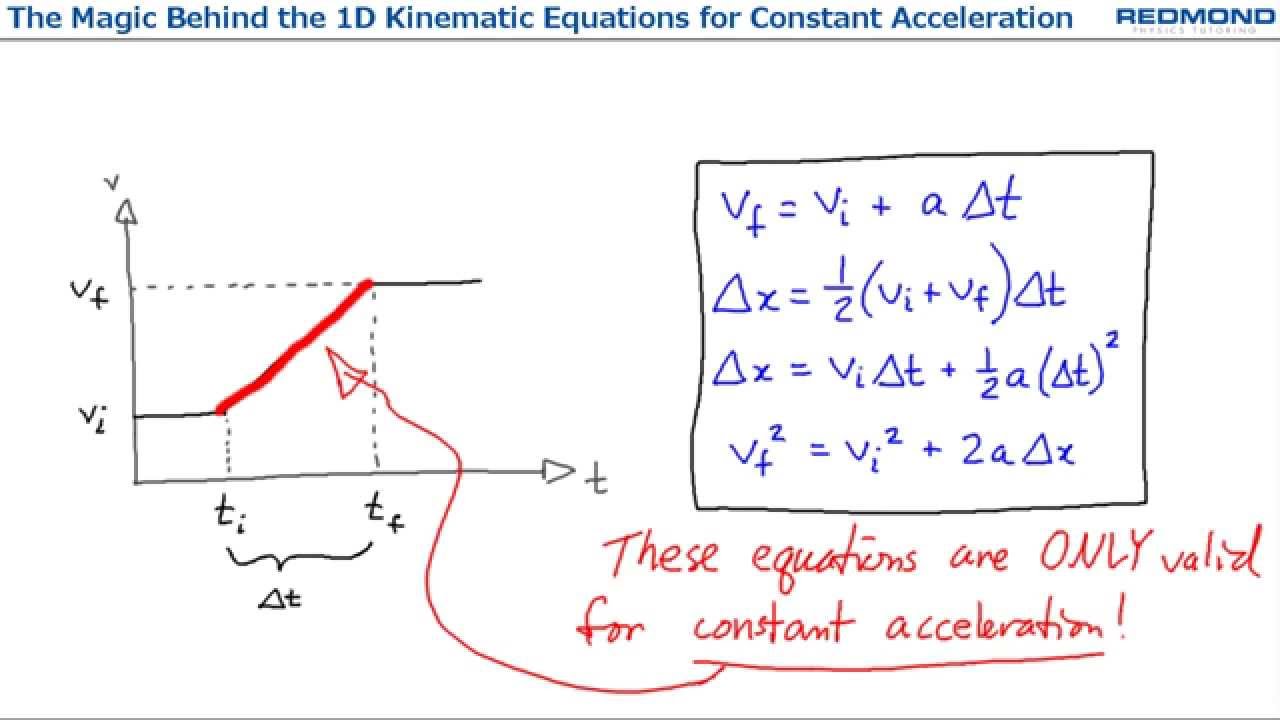
The variables are:

• $\Delta x$: displacement (the change in position, $x_{final}-x_{initial}$)
• $v_0$: initial velocity (velocity at time $t=0$)
• $v$: final velocity
• $a$: constant acceleration
• $t$: time interval

Deriving the Equations from First Principles

You expressed an interest in understanding physics from first principles. The kinematic equations are a perfect example. They aren't just arbitrary formulas; they can be derived directly from the fundamental definitions of velocity and acceleration using calculus.

Velocity is the rate of change of position ($v=ds/dt$), and acceleration is the rate of change of velocity ($a=dv/dt$). By integrating these definitions (the reverse process of finding the rate of change) while holding acceleration constant, we can derive the kinematic equations.

This derivation shows that these equations are a direct mathematical consequence of the definition of constant acceleration. If you're interested in an alternative derivation that uses algebra and the graphical method (calculating the area under the velocity-time graph), the resource "Kinematic Equations" by PASCO scientific has a great walkthrough under the heading "How to Derive the Kinematics Equations," which you can explore later.

How to Choose the Right Equation

Now for the practical part: how do you solve problems with these equations? The key is to pick the right tool for the job. Each equation is missing one of the five variables. Your problem-solving strategy will be:

1. List the variables you know.
2. Identify the variable you want to find.
3. Choose the equation that connects your knowns and your unknown, which is also the equation that ignores the variable you don't know and don't need.

This webpage provides a very clear guide for this strategy.

Let's apply this with a simple example.

Problem: A cart starts from rest and accelerates at a constant $4.0{\text{m/s}}^2$. How fast is it going after it has traveled $5.0$ meters?

Solution Strategy:

1. List knowns:
   • Initial velocity ($v_0$) = 0 m/s ("starts from rest")
   • Acceleration ($a$) = 4.0 m/s²
   • Displacement ($\Delta x$) = 5.0 m
2. Identify unknown:
   • Final velocity ($v$) = ?
3. Choose the equation: We know $v_0,a,\Delta x$ and want $v$. The variable we don't have and don't need is time ($t$). The equation that is "missing time" is: $$v^2=v_0^2+2a\Delta x$$
4. Solve: $$v^2=(0{)}^2+2(4.0{\text{m/s}}^2)(5.0\text{m})$$ $$v^2=40.0{\text{m}}^2/{\text{s}}^2$$ $$v=\sqrt{40.0}\text{m/s}\approx 6.32\text{m/s}$$

Connection to Robotics and Programming

Your interests in robotics and programming are directly tied to these equations.

• Robotics: Imagine a robotic arm on an assembly line that needs to move a component 50 cm in exactly 0.5 seconds. To program the motor controllers, you'd use the kinematic equation $\Delta x=v_{0}t+\frac{1}{2}a{t}^2$ to calculate the precise constant acceleration the arm needs to achieve this task repeatably.
• Programming/Game Development: When you see a character in a video game jump, their vertical motion is governed by these equations. The constant acceleration is gravity ($g=-9.8{\text{m/s}}^2$). The game's physics engine repeatedly calculates the character's new position and velocity in small time steps using these formulas to create a smooth, parabolic arc that looks realistic.

Conclusion

Today we've armed ourselves with the essential tools for describing motion under constant acceleration.

Key Takeaways:

• Constant acceleration means velocity changes at a steady rate, resulting in a linear velocity-time graph and a parabolic position-time graph.
• There are three main kinematic equations that relate displacement, velocity, acceleration, and time.
• These equations can be derived from the fundamental definitions of velocity and acceleration.
• The key to solving problems is to identify your known and unknown variables and select the equation that contains them while ignoring the variable you don't need.

Preview of the Next Lesson:

Now that we have the tools to describe motion, we need to get better at identifying the forces that cause that motion. In the next lesson, we will focus on a critical skill for applying Newton's Laws: constructing free-body diagrams. This will help us visualize all the forces acting on an object, which is the first step toward calculating the net force and, ultimately, the object's acceleration.