Hello! Welcome back to our MBA course.
In our last lesson, we focused on the design of a conjoint analysis study. We learned how to define a business objective and select appropriate attributes and levels to create a survey that effectively captures customer preferences. You designed a study for a hypothetical "Pro" trading platform, breaking the product down into its core components.
Today, we move to the next logical step: making sense of the data once the survey is complete. This lesson addresses the learning outcome: Interpret the output of a conjoint analysis (part-worths, importance scores) to recommend product feature trade-offs.
We will deconstruct the typical outputs of a conjoint study—part-worths and importance scores—and, most importantly, learn how to use them to answer critical business questions. For instance, should we invest in faster execution speed or a better user interface? What price premium can a new feature command? This process translates raw survey data into actionable strategic recommendations.
1. The Core Outputs: Part-Worth Utilities
After respondents complete a conjoint survey, statistical software analyzes their choices to estimate the underlying preference, or utility, for each level of each attribute. These individual preference scores are called part-worths.
The fundamental model assumes that the total utility of a product is simply the sum of the part-worths of its features.
Total Utility (Product) = Part-Worth(Level A) + Part-Worth(Level B) + ...
Let's start by understanding how to read and interpret these part-worths.
Conjoint Analysis methodology, strengths, weaknesses, uses
The following text from 'Conjoint Analysis methodology' explains the concept of part-worths and how they are scaled.
Please read the sections 'Conjoint Analysis' and 'Data Analysis'. Focus on the definitions of utility and part-worth, and the explanation of how a product's total utility is computed by summing the part-worths of its levels.
As the reading mentions, part-worths are typically scaled. A common method is "effects-coding," where the part-worths for all levels within a single attribute sum to zero. This means the zero point represents an average preference, not an absence of utility.
- A positive part-worth indicates a level is more preferred than the average.
- A negative part-worth indicates a level is less preferred than the average.
The following charts show typical outputs for average part-worths from two different studies.
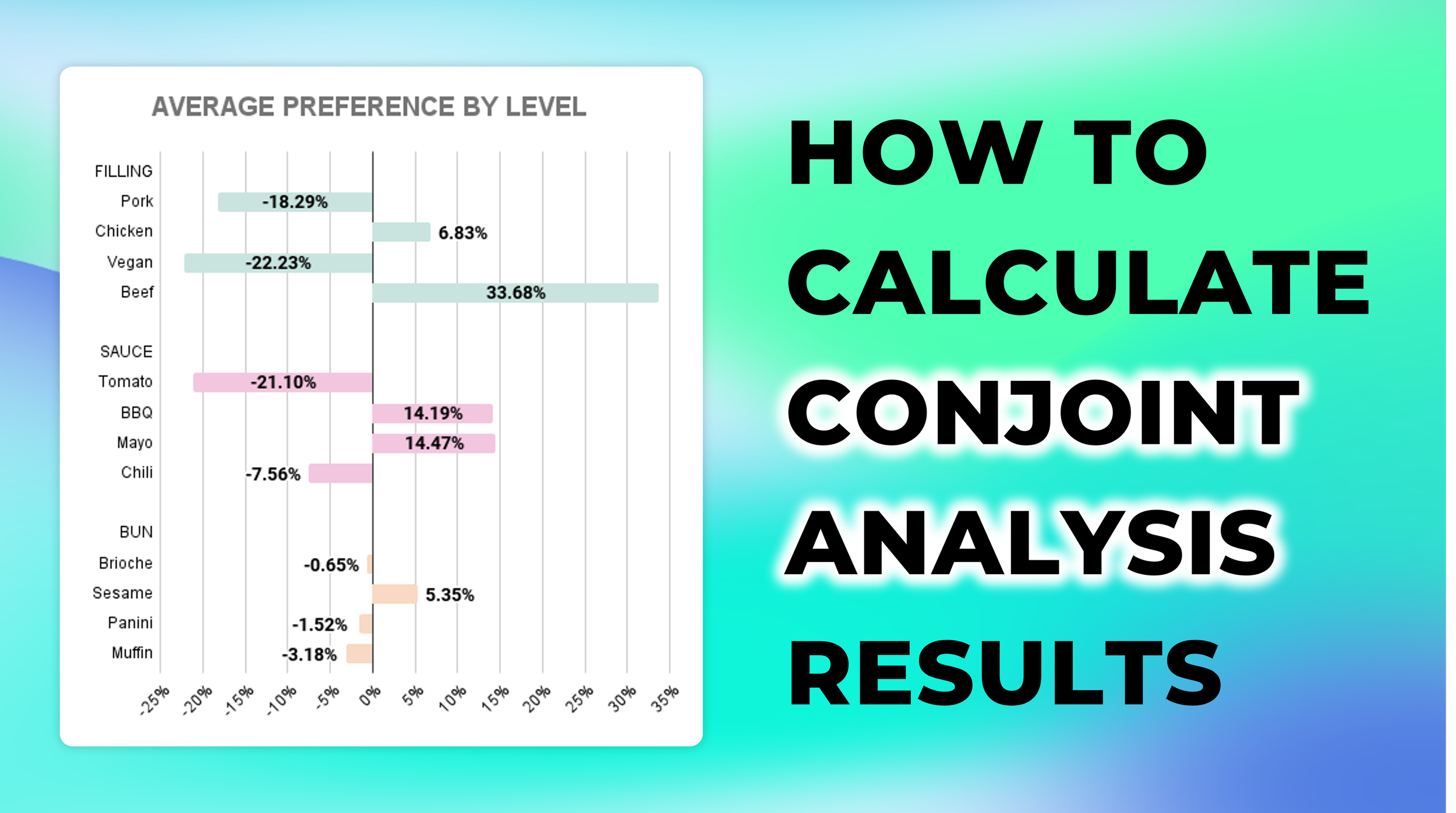

A crucial point for interpretation is that part-worths are interval data, not ratio data. This has important implications.
Interpreting Conjoint Analysis Data
This document, 'Interpreting Conjoint Analysis Data,' provides a more technical and precise explanation of the properties of part-worth utilities.
Please read the first section, 'Conjoint Utilities (Part Worths)'. Pay close attention to why you can compare differences in utility but cannot make ratio comparisons (e.g., 'twice as preferred').
To summarize the key takeaway:
- You can say: "The preference increase from 500MB to 5GB of data is greater than the increase from 5GB to Unlimited."
- You cannot say: "A utility of 20 is twice as good as a utility of 10."
- You cannot directly compare part-worths across different attributes (e.g., you can't say a '$30 price' with a utility of +18.1 is preferred to 'Unlimited data' with a utility of +23.3 in isolation).
2. From Part-Worths to Attribute Importance
While part-worths tell us about the preference for specific levels, we often need a higher-level view: which attributes are most important to customers overall? This is captured by attribute importance scores.
The importance of an attribute is calculated from the range of its part-worths (i.e., the difference between the most preferred and least preferred level). A wider range signifies that the attribute has a greater impact on the consumer's final choice.
Attribute Importance = Max(Part-Worth) - Min(Part-Worth)
These raw importance scores are then typically converted to percentages, showing the relative importance of each attribute, which all sum to 100%.
Conjoint Analysis methodology, strengths, weaknesses, uses
Let's return to the 'Conjoint Analysis methodology' resource to see how importance is calculated and interpreted using the portable projector example.
Read the section 'Attribute Importance' and study Exhibit 10.5. Follow the logic of how the 'Importance' column is calculated from the 'Part-Worth' column, and how that is then converted into 'Relative Importance (%)'.
Let's walk through the calculation for the 'Weight' attribute from Exhibit 10.5:
- Part-worths for Weight: 1.2 kg (+1.5), 1.8 kg (-0.5), 2.4 kg (-1.0)
- Most preferred level: 1.2 kg (Utility = 1.5)
- Least preferred level: 2.4 kg (Utility = -1.0)
- Importance of Weight = 1.5 - (-1.0) = 2.5
To get the relative importance, you sum the importance scores for all attributes (which is 19.53 in the example) and find the percentage for each:
- Relative Importance of Weight = (2.5 / 19.53) * 100% = 12.8%
Unlike part-worths, relative importance scores are ratio data.
Interpreting Conjoint Analysis Data
The 'Interpreting Conjoint Analysis Data' document clarifies the nature of importance scores and offers a key piece of advice for calculating them.
Read the section 'Conjoint Importances'. Note the confirmation that importances are ratio data and the important warning about calculating importances for groups.
This means you can say: "Brand (26.4%) is roughly twice as important as Weight (12.8%) in the customer's decision-making process for this study." This is a powerful and intuitive way to communicate results to stakeholders.
3. Making Recommendations: Trade-Offs and Willingness-to-Pay
This is where conjoint analysis becomes a strategic tool. By understanding the utility values, we can make data-driven recommendations about product feature trade-offs.
Trade-Off Analysis
Product development is a series of trade-offs. Should we add feature X, which costs $10 in R&D, or feature Y, which costs $15? Conjoint analysis allows us to quantify the customer value side of this equation.
Conjoint Analysis methodology, strengths, weaknesses, uses
The 'Conjoint Analysis methodology' resource provides a clear example of how to perform a trade-off analysis.
Read the short section 'Trade-off Analysis' and examine Exhibit 10.6. Understand how the change in utility is calculated for two different potential product improvements.
The logic is straightforward: calculate the utility gain from each potential improvement and recommend the one that delivers more value to the customer.
- Improving Brightness (2000 -> 3000 lumens): Utility gain = 1.48 - 0.52 = +0.96
- Reducing Weight (1.8kg -> 1.2kg): Utility gain = 1.5 - (-0.5) = +2.0
- Recommendation: Customers value the weight reduction more than the brightness improvement.
Willingness-to-Pay (WTP)
A powerful extension of this is to monetize the utility of features. By using Price as an attribute, we can calculate how much more customers would be willing to pay for a specific improvement. This is a direct input for pricing strategy.
Conjoint Analysis methodology, strengths, weaknesses, uses
Finally, let's see how to calculate a price premium for a new feature.
Read the final paragraphs under the 'Price' section, starting from 'Traditional conjoint analysis is appropriate for answering questions such as what to charge for a product feature.' Follow the calculation for the price premium of the lighter projector model.
The method is as follows:
- Calculate the utility gain from the new feature (e.g., utility gain from weight reduction = 2.0).
- Calculate the utility change per dollar. From the example, the price range is $600 ($1200 - $600) and the utility range is 3.06 (1.53 - (-1.53)). This gives a "value" of 3.06 utility points per $600, or 0.0051 utility points per dollar.
- Monetize the feature's utility gain. The value of the weight reduction is its utility gain divided by the utility-per-dollar rate: 2.0 / 0.0051 ≈ $392.
- Recommendation: The company can charge a price premium of approximately $400 for the lighter model.
4. Application Exercise
Let's return to the "Pro" trading platform study you designed in the last lesson. Assume you've run the study and received the following average part-worth utilities.
| Attribute | Level | Part-Worth Utility |
|---|---|---|
| Monthly Fee | $15/month | 15 |
| $45/month | 5 | |
| $99/month | -20 | |
| Execution Speed | Standard (100-200ms) | -18 |
| Fast (20-50ms) | 8 | |
| Ultra-Low Latency (<5ms) | 10 | |
| API Access | No API Access | -12 |
| Market Data API Only | 2 | |
| Full Trading API | 10 | |
| Advanced Charting | Standard Charting | -7 |
| Pro Charting | 7 | |
| Customer Support | Email & Chatbot | -11 |
| 24/7 Live Chat | 4 | |
| Dedicated Account Manager | 7 |
Your Task: Based on this data, answer the following questions for your management team.
- Calculate the relative importance of each of the five attributes. Which attribute is the most important driver of choice for your target users?
- Trade-off Decision: Your engineering team can either upgrade Execution Speed from 'Fast' to 'Ultra-Low Latency' OR upgrade Customer Support from '24/7 Live Chat' to a 'Dedicated Account Manager'. Which initiative should you prioritize to deliver the most value to customers?
- Willingness-to-Pay: What is the maximum monthly price premium customers would be willing to pay for an upgrade from 'Standard Charting' to 'Pro Charting'?
Click to see the solution
1. Relative Importance Calculation
| Attribute | Max Utility | Min Utility | Importance (Range) | Relative Importance |
|---|---|---|---|---|
| Monthly Fee | 15 | -20 | 35 | 39.3% |
| Execution Speed | 10 | -18 | 28 | 31.5% |
| API Access | 10 | -12 | 22 | 24.7% |
| Advanced Charting | 7 | -7 | 14 | 15.7% |
| Customer Support | 7 | -11 | 18 | 20.2% |
| Total | 117 | 100% |
Correction after summing: The total importance is 35+28+22+14+18 = 117. Let's re-calculate percentages.
| Attribute | Importance | Relative Importance |
|---|---|---|
| Monthly Fee | 35 | 35/117 = 29.9% |
| Execution Speed | 28 | 28/117 = 23.9% |
| API Access | 22 | 22/117 = 18.8% |
| Advanced Charting | 14 | 14/117 = 12.0% |
| Customer Support | 18 | 18/117 = 15.4% |
| Total | 117 | 100% |
Answer: Monthly Fee is the most important attribute (29.9%), followed closely by Execution Speed (23.9%). This indicates users are highly sensitive to both price and performance.
2. Trade-off Decision
- Option A (Speed Upgrade): Utility gain = Utility(Ultra-Low) - Utility(Fast) = 10 - 8 = +2 points.
- Option B (Support Upgrade): Utility gain = Utility(Dedicated) - Utility(24/7 Chat) = 7 - 4 = +3 points.
Recommendation: Prioritize the upgrade to a 'Dedicated Account Manager'. It delivers a higher utility gain to customers than the final speed improvement.
3. Willingness-to-Pay for Pro Charting
- Utility Gain from Pro Charting:
- Utility(Pro) - Utility(Standard) = 7 - (-7) = 14 points.
- Utility per Dollar:
- The price range is $99 - $15 = $84.
- The utility range for price is 15 - (-20) = 35 points.
- Utility per dollar = 35 points / $84 ≈ 0.417 points per dollar.
- Monetize the Feature:
- Value of Pro Charting = (Utility Gain) / (Utility per Dollar) = 14 / 0.417 ≈ $33.57.
Recommendation: Customers are willing to pay a premium of approximately $34 per month for the 'Pro Charting' tools. This can be used to inform the pricing of a feature bundle or a higher subscription tier.
Conclusion
In this lesson, we translated the abstract choices of survey respondents into a concrete, quantitative framework for making product and pricing decisions. You are now equipped to not only design a conjoint study but also to interpret its results and deliver strategic recommendations.
Key Takeaways:
- Part-worths are interval-level scores that quantify customer preference for each feature level. The total utility of a product is the sum of its part-worths.
- Attribute importance is a ratio-level score derived from the range of part-worths, indicating which product attributes have the most influence on customer choice.
- By comparing the change in utility from different feature improvements, we can make informed trade-off decisions.
- By establishing a relationship between utility and price, we can calculate customers' willingness-to-pay for specific features, directly informing pricing strategy.
This concludes our deep dive into conjoint analysis. In our next module, we will shift from marketing analytics to the core of the business engine: Operations and Process Management. We will begin by learning how to apply quantitative forecasting methods to predict demand—a critical input for any operational plan.