Introduction
Welcome to the first lesson of our final module. In our previous session, we compared Logistic Regression and XGBoost, ultimately selecting XGBoost as our champion model due to its superior predictive performance on key metrics like ROC-AUC and Recall. We acknowledged, however, that its power comes with the challenge of being a "black box."
This lesson brings us to the crucial step of refining our model from a purely statistical tool into a business-aligned asset. We will address this learning outcome: Perform a comprehensive evaluation of the selected model, including classification threshold tuning based on business cost considerations.
We'll move beyond the standard 0.5 probability cutoff and learn how to select a decision threshold that explicitly minimizes financial risk and maximizes value for the lending institution. As noted by Professor Bart Baesens, a leading expert in credit risk analytics, evaluating models on profitability and business impact is just as important as statistical performance.
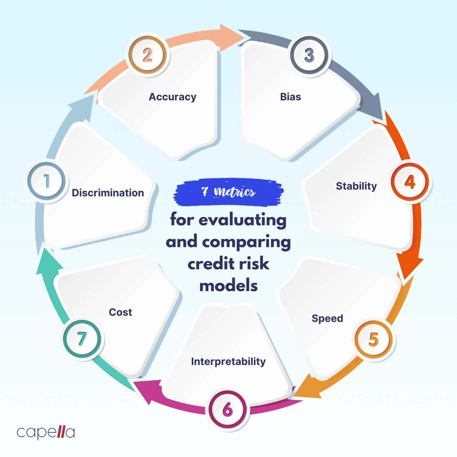
By the end of this lesson, you will be able to translate abstract model probabilities into concrete, justifiable business decisions.
1. Why the Default Threshold is a Business Risk
When we use a classifier's .predict() method, it typically uses a default probability threshold of 0.5. Any prediction with a probability of default > 0.5 is classified as a default (1), and anything <= 0.5 is classified as non-default (0).
This 50/50 split is often arbitrary and rarely optimal in a real-world business setting. It implicitly assumes that the cost of a False Positive is the same as the cost of a False Negative. In our loan default scenario, this assumption is dangerously wrong.
To understand why, let's analyze the costs associated with each type of error.
Confusion Matrix Components and Error Costs
This section of the 'Credit Risk Modeling in Python' article clearly explains the asymmetrical cost of prediction errors in a lending context.
Please read the subsection under 'Confusion Matrix' that begins 'In this context of Credit Risk Analysis...'. Focus on the example financial impacts of a False Positive versus a False Negative.
As the article makes clear:
- False Negative (FN): We predict 'non-default', but the customer does default. Cost: High. The bank loses the entire principal of the loan, plus administrative costs.
- False Positive (FP): We predict 'default', but the customer would have paid it back. Cost: Low. The bank loses out on the potential interest income from that single loan.
Losing the entire loan amount is far worse than losing potential interest. Therefore, our evaluation and decision-making process must reflect this cost imbalance. By adjusting the classification threshold, we can tune the model's behavior to be more cautious, thereby minimizing the number of costly False Negatives.
2. Strategy 1: Simulation to Maximize Business Value
One powerful way to find an optimal threshold is to simulate the business impact of various threshold choices. We can create a "strategy table" that explores how changing our loan acceptance criteria affects key business indicators.
This involves introducing a few business-centric metrics:
- Acceptance Rate: The percentage of loan applications that our model approves. A lower threshold means we are stricter, approving fewer people, leading to a lower acceptance rate.
- Bad Rate: The percentage of approved loans that end up defaulting. This is our primary risk indicator.
- Estimated Value: A simulated profit/loss calculation based on the number of accepted loans, the bad rate, and the average loan amount. This metric directly estimates the financial outcome of our strategy.
The following resource provides a superb walkthrough of this entire simulation process, from defining the metrics to creating and interpreting the final results.
Credit Risk Modeling in Python
This article provides a practical, step-by-step guide to connecting model thresholds to business KPIs. We'll use its methodology to build a strategy table.
Please read the sections titled 'Acceptance Rate', 'Bad Rate', 'Exploring a Range of Possibilities', 'Estimated Value', and 'Some analysis'. Focus on how the author creates a table (strat_df) to simulate the impact of different acceptance rates on key business metrics like Bad Rate and Estimated Value.
The Core Logic
The analysis you just read follows these steps:
- Use the trained XGBoost model to get the predicted probabilities of default for the test set.
- Define a range of potential
Acceptance Ratesto test (e.g., from 95% down to 5%). - For each
Acceptance Rate, calculate the corresponding probabilitythreshold. For example, an acceptance rate of 80% means we approve the 80% of applicants with the lowest predicted probability of default. The threshold is the highest probability within this approved group. - Apply this threshold to classify applicants as 'accepted' or 'rejected'.
- For the 'accepted' group, calculate the
Bad Rate(the actual default rate within this group) and theEstimated Value. - Plot
Estimated Valuevs.Acceptance Rateto find the peak. This peak represents the strategy that maximizes our simulated financial return, and it gives us the optimal threshold to use.
The chart of "Estimated Value by Acceptance Rate" in the article is the key deliverable of this analysis. It provides a clear, data-driven recommendation for the business on which threshold to adopt to maximize profitability.
3. Strategy 2: Automated Cost-Sensitive Tuning
While simulation is intuitive, a more direct and automated approach is to define a custom scoring function that represents our business costs and then use a tool to find the threshold that optimizes it. scikit-learn provides an excellent tool for this: TunedThresholdClassifierCV.
First, we need to create a function that calculates a "score" based on our cost matrix. We want to maximize this score. Let's assign a "gain" to each outcome:
- True Negative (TN): Approved a good loan. Gain =
+ interest(for simplicity, we can ignore this and set it to 0, focusing only on costs). - True Positive (TP): Correctly rejected a bad loan. Gain =
0. - False Positive (FP): Rejected a good loan. Gain =
-1(representing the lost opportunity cost). - False Negative (FN): Approved a bad loan. Gain =
-5(representing a much larger loss).
The scikit-learn documentation provides a perfect template for this.
Post-tuning the decision threshold for cost-sensitive learning
The scikit-learn documentation provides a clear example of how to define a cost-matrix and use a dedicated tool for finding the optimal threshold.
Read the section 'Cost-sensitive learning with constant gains and costs'. Pay close attention to how the credit_gain_score function is created using a gain_matrix and then used with TunedThresholdClassifierCV.
Now that you understand how to define the cost function, let's see how to apply it efficiently. Since we have already trained our XGBoost model in the previous lesson, we don't need to retrain it repeatedly during the threshold search. We can use the cv='prefit' option.
Automatically tuning thresholds
This video provides a concise visual walkthrough of using TunedThresholdClassifierCV and highlights the efficient 'prefit' strategy.
Watch from 03:22 to 04:48 to see how TunedThresholdClassifierCV is instantiated. Then, pay close attention to the segment from 06:43 to 08:42, which explains the cv='prefit' and refit=False settings. This is exactly the approach we'll use.
Implementation
Here's how you would implement this with our trained XGBoost model.
import numpy as np
from sklearn.metrics import make_scorer, confusion_matrix
from sklearn.model_selection import TunedThresholdClassifierCV


# Assume 'xgb_model' is your trained XGBoost classifier from the previous lesson
# Assume 'X_val', 'y_val' is a validation set held out for tuning the threshold


# 1. Define the custom scoring function based on our cost matrix
def credit_gain_scorer(y_true, y_pred, **kwargs):
    cm = confusion_matrix(y_true, y_pred)


    # Gain Matrix: [[TN, FP], [FN, TP]]
    # We define gains as: TN=0, TP=0, FP=-1, FN=-5
    gain_matrix = np.array([[0, -1], [-5, 0]])
    return np.sum(cm * gain_matrix)


# Make it a scikit-learn scorer
business_scorer = make_scorer(credit_gain_scorer, greater_is_better=True)


# 2. Use TunedThresholdClassifierCV on the pre-trained model
# We use a validation set (X_val, y_val) to find the threshold to avoid overfitting.
tuned_xgb = TunedThresholdClassifierCV(
    estimator=xgb_model,          # Our already trained XGBoost model
    scoring=business_scorer,      # The business metric to maximize
    cv="prefit",                  # IMPORTANT: Tells it not to re-train the estimator
    refit=False,                  # We don't need to refit the final model
    store_cv_results=True
)


# Fit it on the validation data to find the best threshold
tuned_xgb.fit(X_val, y_val)


# 3. Analyze the results
print(f"Optimal threshold based on business cost: {tuned_xgb.best_threshold_:.4f}")


# Compare the score with the default 0.5 threshold vs. the tuned one
default_preds = (xgb_model.predict_proba(X_val)[:, 1] > 0.5).astype(int)
tuned_preds = tuned_xgb.predict(X_val)

print(f"Business score with default 0.5 threshold: {credit_gain_scorer(y_val, default_preds)}")
print(f"Business score with optimal threshold: {credit_gain_scorer(y_val, tuned_preds)}")
You would find that the optimal threshold is likely much lower than 0.5 (e.g., 0.2-0.3). This means the model becomes much stricter, flagging more applicants as potential defaults. While this increases False Positives, it significantly cuts down on the very costly False Negatives, leading to a better overall business score (a smaller loss).
Conclusion
In this lesson, we elevated our model evaluation from a purely statistical exercise to a business-centric optimization process. You learned how to align your model's decision-making with the financial realities of the business problem.
Key Takeaways:
- The Default Threshold is Arbitrary: The standard 0.5 probability threshold is rarely optimal for business problems with asymmetric costs.
- Threshold Tuning is a Business Lever: Adjusting the classification threshold is a powerful way to control the trade-off between risk and opportunity (e.g., False Negatives vs. False Positives).
- Connect to Business KPIs: Techniques like simulation (strategy tables) and custom cost functions allow you to translate model performance directly into business metrics like profit, loss, or risk exposure.
- Automate with the Right Tools:
scikit-learn'sTunedThresholdClassifierCVprovides an efficient, robust way to find an optimal threshold based on a custom, cost-sensitive metric.
Next Steps:
We have now selected our final model (XGBoost) and optimized its decision threshold to maximize business value. However, it remains a "black box." For a bank to trust and deploy this model, especially in a regulated environment, they need to understand why it makes certain decisions.
In our next and final lesson, Generate and interpret model explanations (e.g., using SHAP) to communicate key risk drivers to business stakeholders, we will learn how to open this black box and extract actionable insights, making our model not just predictive, but also explainable.