Introduction
Welcome to the third lesson in our project. In our last session, we constructed a robust modeling pipeline that correctly incorporates the SMOTE technique to handle class imbalance, preventing the common pitfall of data leakage. We established this pipeline using a LogisticRegression model as our initial classifier and validated its performance with cross-validation.
Today, we will move from building the infrastructure to the crucial stage of model selection. This lesson directly addresses the learning outcome: to train and compare a baseline model (Logistic Regression) with a complex model (XGBoost) to select the final model based on our pre-defined evaluation metrics.
This is a standard and critical phase in any data science project. We will not just look for the model with the highest score. Instead, we will perform a professional, multi-faceted comparison, weighing performance gains against trade-offs in interpretability, complexity, and computational cost—all within the context of our loan default prediction scenario.
1. Choosing the Contenders: A Tale of Two Models
In machine learning, it's a best practice to start with a simple, interpretable baseline model before moving to more complex ones. This approach helps you understand the data better and establishes a performance benchmark to beat.
Our Baseline: Logistic Regression (LR)
As you know, Logistic Regression is a linear model. Its strength lies in its simplicity, speed, and high interpretability. The model's coefficients directly tell us the relationship between each feature and the log-odds of the outcome. In a regulated industry like finance, being able to explain why a decision was made is often a requirement, making LR a powerful and common choice. We've already implemented it within our SMOTE pipeline.
Our Challenger: XGBoost (Extreme Gradient Boosting)
XGBoost is a highly sophisticated and powerful algorithm based on gradient boosted decision trees. It has a reputation for achieving state-of-the-art results on tabular data. It excels at capturing complex, non-linear relationships and interactions between features automatically, something LR can only do if you manually engineer those features. This power, however, comes at the cost of being a more "black box" model, making its decisions harder to interpret directly.
To understand the practical trade-offs between these two models, please read the following article.
XGBoost vs Logistic Regression
This article from Medium provides a great, practitioner-focused comparison of XGBoost and Logistic Regression.
Please read Section 2 'Key Differences' and Section 3 'When to Use XGBoost vs Logistic Regression?'. Focus on the discussion around feature engineering, handling non-linearity, and the interpretability vs. performance trade-off.
The article highlights a key tension: LR's interpretability vs. XGBoost's power. In a loan application scenario, this is not a trivial choice. Watch this short clip for a pointed discussion on this exact topic.
This video from Super Data Science discusses when XGBoost might not be the best choice. The beginning of the clip is highly relevant to our loan default problem.
Watch from 00:14 to 03:18. Pay attention to the argument about model interpretability in the context of loan application decisions.
As you can see, selecting a model isn't just a technical exercise; it's a business decision. We'll keep this trade-off in mind as we evaluate their performance.
2. Implementation: Running the Comparison
We will now use the imblearn pipeline we built in the previous lesson to train and evaluate both models on our preprocessed training data. This ensures a fair, "apples-to-apples" comparison, as both models will benefit from the same SMOTE-based resampling.
Let's assume our data is already split into X_train, X_test, y_train, y_test, and our feature engineering/scaling has been performed.
Here is the Python code to set up and run the evaluation for both models using cross_val_score. This process rigorously tests how well each model is likely to generalize to unseen data.
import pandas as pd
from sklearn.model_selection import StratifiedKFold, cross_val_score
from imblearn.pipeline import Pipeline as ImbPipeline
from imblearn.over_sampling import SMOTE
from sklearn.linear_model import LogisticRegression
from xgboost import XGBClassifier
import numpy as np


# Assume X_train, y_train are your prepared training data


# --- 1. Define the Logistic Regression Pipeline ---
lr_pipeline = ImbPipeline([
    ('smote', SMOTE(random_state=42)),
    ('classifier', LogisticRegression(random_state=42, solver='liblinear'))
])


# --- 2. Define the XGBoost Pipeline ---
# Note: We set 'use_label_encoder=False' and 'eval_metric' to avoid deprecation warnings
xgb_pipeline = ImbPipeline([
    ('smote', SMOTE(random_state=42)),
    ('classifier', XGBClassifier(random_state=42, use_label_encoder=False, eval_metric='logerror'))
])


# --- 3. Define Cross-Validation Strategy ---
cv = StratifiedKFold(n_splits=5, shuffle=True, random_state=42)


# --- 4. Evaluate Both Pipelines ---
# We will use 'roc_auc' as it's a good overall metric for classification,
# and 'recall_macro' to check performance on our rare default class.
scoring = ['roc_auc', 'recall_macro']


# Evaluate Logistic Regression
lr_scores = cross_val_score(lr_pipeline, X_train, y_train, scoring='roc_auc', cv=cv, n_jobs=-1)
print(f"Logistic Regression ROC-AUC (CV): {np.mean(lr_scores):.4f} +/- {np.std(lr_scores):.4f}")


# Evaluate XGBoost
xgb_scores = cross_val_score(xgb_pipeline, X_train, y_train, scoring='roc_auc', cv=cv, n_jobs=-1)
print(f"XGBoost ROC-AUC (CV): {np.mean(xgb_scores):.4f} +/- {np.std(xgb_scores):.4f}")
After running cross-validation, we would train the final models on the full training set to evaluate them on the hold-out test set (X_test, y_test). This gives us our final performance numbers.
3. Comparative Analysis and Model Selection
With the results from our models, we can now conduct a comparative analysis. This involves more than just looking at one number. We'll use a combination of metrics and visualizations.
To see an excellent example of how this is done in a credit risk context, please review the following article.
A Machine Learning Approach To Credit Risk Assessment
This Towards Data Science article walks through a credit risk assessment project, including a section on comparing different models.
Please read Section 4, 'Model training and evaluation'. Focus on how the author uses a classification report, ROC curves, and AUC scores to compare KNN, Logistic Regression, and XGBoost.
Key Comparison Points:
1. Classification Metrics (Precision, Recall, F1-Score)
After training on the full X_train, we would generate a classification_report for each model on the X_test.
- For the bank, a False Negative is most costly: This is when we predict a client will not default, but they do. We lose the entire loan amount. This means Recall for the 'default' class (class 1) is a critical metric.
- False Positives also have a cost: This is predicting a client will default, but they would have paid it back. We lose the potential interest income. This relates to Precision.
We are looking for the model that gives us the best balance, but with a strong emphasis on high Recall for the default class.
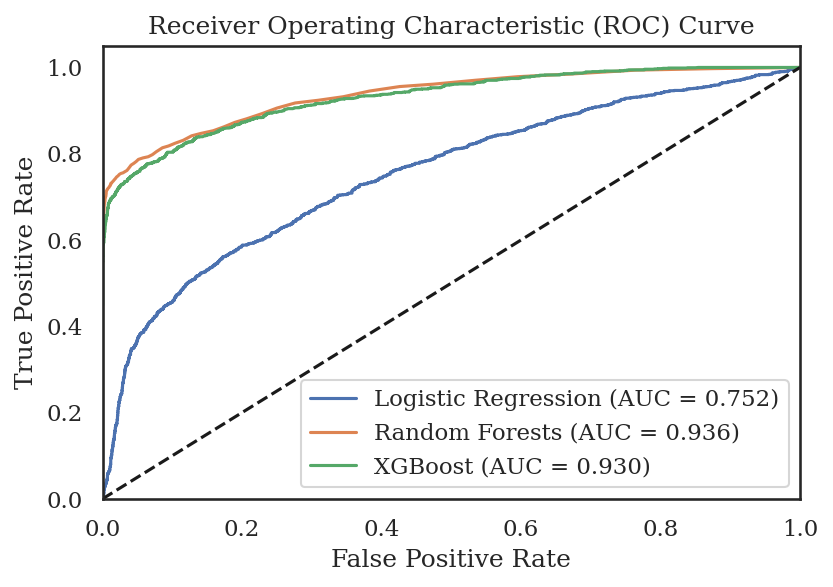
2. ROC Curve and AUC Score
The ROC curve is one of the most important tools for comparing binary classifiers. It plots the True Positive Rate (Recall) against the False Positive Rate at all classification thresholds. The Area Under the Curve (AUC) summarizes this plot into a single number. A higher AUC means the model is better at distinguishing between the positive and negative classes.
Making the Decision
Let's assume our analysis yields the following hypothetical results:
| Metric | Logistic Regression | XGBoost | Justification |
|---|---|---|---|
| AUC Score | 0.78 | 0.86 | XGBoost is significantly better at distinguishing defaulters from non-defaulters. |
| Recall (Default) | 0.65 | 0.75 | XGBoost correctly identifies 10% more of the actual defaulters. |
| Precision (Default) | 0.55 | 0.52 | LR is slightly better at being right when it predicts a default. |
| F1-Score (Default) | 0.59 | 0.61 | The harmonic mean of P & R shows XGBoost has a slightly better balance. |
| Interpretability | High | Low | LR coefficients are easy to explain; XGBoost decisions are complex. |
| Training Time | Fast | Slow | LR trains in seconds; XGBoost can take minutes. |
In this scenario, XGBoost offers a substantial improvement in identifying defaulters (Recall) and overall discriminatory power (AUC). This performance gain likely outweighs its lower interpretability and longer training time, especially since training is an offline process. The slightly lower precision is a trade-off we might be willing to make to catch more defaults.
Therefore, we select XGBoost as our champion model. We acknowledge its "black box" nature as a challenge that we will address in the next and final lesson.
Conclusion
In this lesson, we formalized the process of model selection, a cornerstone of professional data science work.
Key Takeaways:
- Establish a Baseline: Always start with a simple, interpretable model like Logistic Regression to set a performance benchmark.
- Compare on Multiple Fronts: Model selection is not about a single metric. It's a strategic decision that balances predictive performance (AUC, Recall), business needs (interpretability), and operational constraints (training time).
- Fair Comparison is Key: Using a consistent pipeline (including resampling and preprocessing) for all candidate models ensures that you are comparing the models themselves, not the artifacts of your workflow.
- XGBoost often wins on performance for tabular data due to its ability to model complex non-linearities, but this comes at the cost of being less transparent.
Next Steps:
We have selected XGBoost as our final model. However, our work isn't done. A "black box" model with high performance is useful, but a model that is high-performing and explainable is invaluable. In our final lesson, Interpretation, Reporting, and Deployment Strategy, we will tackle two critical tasks:
- Fine-tuning the model's classification threshold to align with business costs.
- Using powerful techniques like SHAP (SHapley Additive exPlanations) to open the "black box" and explain XGBoost's predictions to business stakeholders.