Multi-Layer Perceptron: Forward and Backward Propagation

1. Setting the Stage: Network Structure and Initialization

Before we can propagate anything, we need a network. We'll structure our implementation logically with separate functions for initialization, forward pass, and backward pass.

Initializing Parameters

A neural network's parameters—weights ($W$) and biases ($b$)—must be initialized before training begins. A common strategy is to initialize the weights with small random numbers. This breaks the symmetry between neurons and ensures they learn different features. Biases can be initialized to zero or small random numbers.

The dimensions of the weight matrices are critical. For a connection between layer $l-1$ with $n^{[l-1]}$ neurons and layer $l$ with $n^{[l]}$ neurons, the weight matrix $W^{[l]}$ will have the shape (n_neurons_current_layer, n_neurons_previous_layer), or $(n^{[l]},n^{[l-1]})$. The bias vector $b^{[l]}$ will have the shape $(n^{[l]},1)$.

To see a clean implementation of this, let's watch a short video segment.

2. The Forward Pass: From Input to Prediction

The forward pass is the process of taking an input and feeding it through the network layer by layer to get a prediction. Given your background, the most efficient way to think about this is in terms of matrix operations.

For each layer $l$:

1. Calculate the pre-activation: $Z^{[l]}=W^{[l]}{A}^{[l-1]}+B^{[l]}$
2. Calculate the activation: $A^{[l]}=\sigma (Z^{[l]})$

Here, $A^{[l-1]}$ is the matrix of activations from the previous layer, where each column is a separate training example. This vectorized approach allows us to process an entire batch of data at once using NumPy's efficient matrix multiplication (.dot() or @).

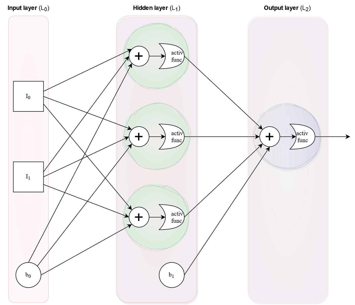
It's crucial to cache the intermediate values ($Z^{[l]}$ and $A^{[l]}$) during the forward pass. We will need them for the backward pass calculations.

Let's see this implemented in code.

3. The Backward Pass: Calculating Gradients

This is where we implement the four equations we derived. We start from the final layer and work our way backward, calculating the gradient of the loss with respect to each parameter.

The process for a single training batch is:

1. Compute the output error (${\delta }^{[L]}$): This is the first step of backpropagation. It tells us how much the pre-activation of the output layer contributed to the final loss. The calculation depends on your loss function. For MSE, the derivative of the loss term ${\nabla }_{a}L$ is simply $(A^{[L]}-Y)$.
2. Calculate gradients for the output layer ($d{W}^{[L]},d{b}^{[L]}$): Using ${\delta }^{[L]}$ and the cached activation from the previous layer $A^{[L-1]}$, we apply our gradient equations.
3. Propagate the error to the previous layer: We calculate ${\delta }^{[L-1]}$ using ${\delta }^{[L]}$ and the weights $W^{[L]}$.
4. Calculate gradients for the hidden layer ($d{W}^{[L-1]},d{b}^{[L-1]}$): Using the new ${\delta }^{[L-1]}$ and its corresponding input activation $A^{[L-2]}$.
5. Repeat this process until we reach the first layer.

To get a complete, end-to-end view of both the forward and backward passes implemented together, the following tutorial is excellent. It's a bit longer, but it walks through the entire logic with code.

The article below provides the same logic but in a clean, object-oriented Python class. It's an excellent reference to read through, as the code is a direct translation of the backpropagation equations.

4. The Grand Finale: The Training Loop

Now we assemble the pieces. A training loop for a neural network does the following for a set number of epochs (passes over the entire dataset):

1. Iterate through the training data in batches.
2. For each batch:
   a. Perform the forward pass to get the predictions and cached values.
   b. Compute the loss.
   c. Perform the backward pass to compute the gradients ($dW,db$).
   d. Update the parameters using gradient descent:
   $W^{[l]}=W^{[l]}-\alpha \cdot d{W}^{[l]}$
   $b^{[l]}=b^{[l]}-\alpha \cdot d{b}^{[l]}$
3. Optionally, evaluate the model on a validation set to monitor progress.

The Dataquest video you watched shows a complete, runnable training loop that puts everything together.

Conclusion

Congratulations! You have now walked through the complete implementation of a neural network's training algorithm from scratch. This is a formidable and hugely important exercise.

Key Takeaways:

• Forward Propagation is a sequence of matrix multiplications and non-linear activations, flowing from input to output. Caching intermediate values is essential.
• Backward Propagation is an algorithm that computes gradients by propagating an error signal backward, from the output to the input.
• The core of backprop involves calculating an error term $\delta$ for each layer and using it to find the gradients for that layer's weights and biases.
• The Training Loop orchestrates the entire process by repeatedly calling the forward pass, backward pass, and updating the parameters using the computed gradients.

You've bridged the gap between the abstract math of our last lesson and the concrete reality of code. This gives you a powerful mental model for what happens every time you call model.train() in a high-level framework.

Preview of the Next Lesson:
We've built the engine of our neural network. Now, we need to tune it. In the next lesson, we will explore some of the critical components we used today: "Explain the role of various activation functions (e.g., ReLU, Sigmoid) and weight initialization strategies." We've seen ReLU in action, but why is it so popular? Are there better choices? How can smart initialization make our network train faster and more reliably? We'll answer these questions next.