Activation Functions & Weight Initialization

1. The Role of Activation Functions

In the network you built, the activation function was the non-linear step ($\sigma$) applied after the linear transformation ($Z=WX+B$). But why is this non-linearity so important?

Without an activation function (or with a "linear" activation function, $f(x)=x$), a neural network, no matter how many layers it has, is just a stack of linear operations. A sequence of linear transformations can always be collapsed into a single linear transformation. This means your "deep" network would be no more powerful than a simple linear regression model, incapable of learning the complex, non-linear patterns found in data like images, text, or economic trends.

Activation functions are the key that unlocks the expressive power of neural networks. Let's start with a video that explains this fundamental concept.

A Tour of Common Activation Functions

Now that you understand their purpose, let's explore the zoo of popular activation functions. Each has distinct properties that affect how a network learns.

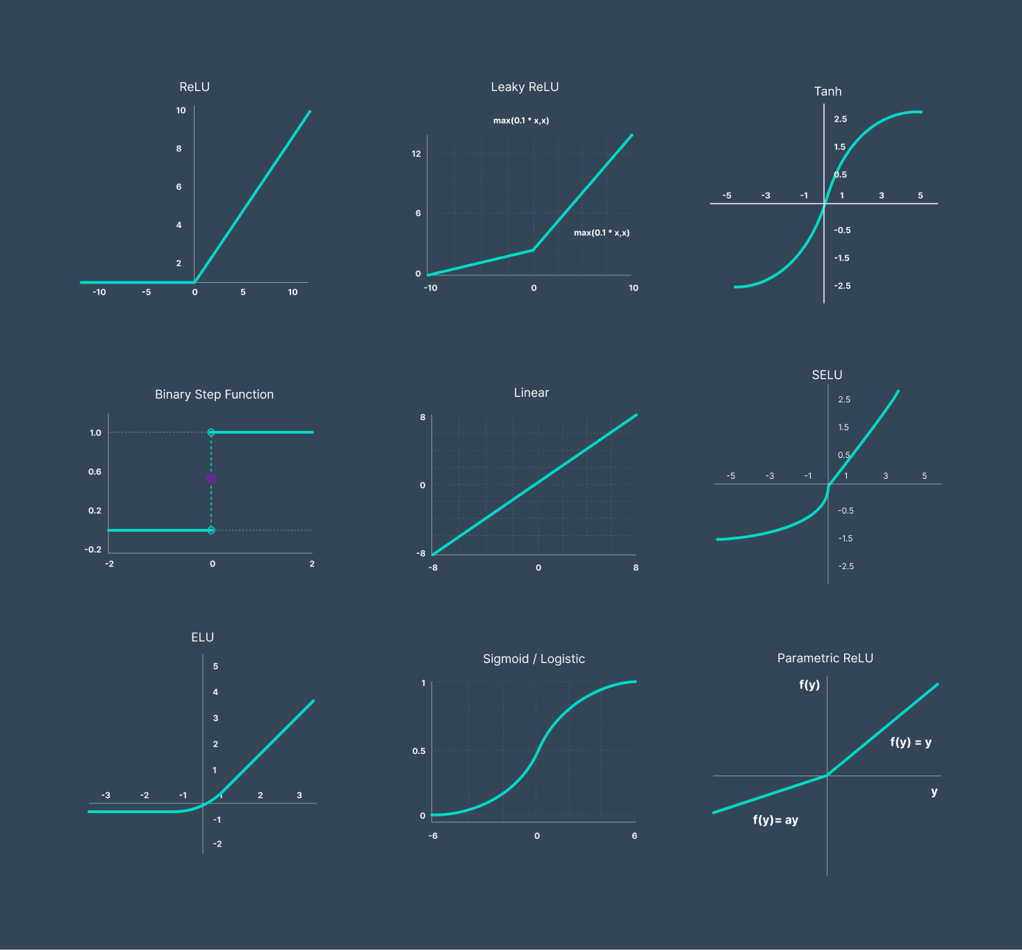
To get a hands-on feel for these functions, their gradients, and their impact on training, we'll use a fantastic interactive notebook from the University of Amsterdam's Deep Learning course.

Let's summarize the key players and their characteristics:

• Sigmoid ($\sigma (x)=\frac{1}{1+e^{-x}}$):

  • Pros: Squashes numbers to a probability-like range of [0, 1]. Historically popular and useful in the output layer for binary classification.
  • Cons: Suffers from the vanishing gradient problem. As you can see from its gradient plot, for very large or very small inputs, the gradient is almost zero. In deep networks, this can cause the gradients flowing back to the early layers to become vanishingly small, effectively halting learning. Also, its output is not zero-centered.

• Tanh (Hyperbolic Tangent):

  • Pros: Squashes numbers to [-1, 1]. Its output is zero-centered, which can help with optimization.
  • Cons: Like Sigmoid, it saturates at the extremes and suffers from the vanishing gradient problem.

• ReLU (Rectified Linear Unit, $f(x)=\max (0,x)$):

  • Pros: The current default for hidden layers. It's computationally very efficient. It does not saturate for positive inputs, which means it doesn't suffer from vanishing gradients on that side. This property greatly accelerates the convergence of SGD.
  • Cons: The "Dying ReLU" problem. If a neuron's input is always negative, it will always output zero. Consequently, the gradient flowing through it will forever be zero. The neuron "dies" and plays no further part in learning.

• Leaky ReLU, ELU, Swish:

  • These are all variants designed to solve the Dying ReLU problem by ensuring the function has a small, non-zero gradient for negative inputs.
  • Leaky ReLU: Introduces a small slope for negative values (e.g., $0.01x$).
  • ELU (Exponential Linear Unit): Uses an exponential curve for negative values.
  • Swish: A smooth function that is non-monotonic, sometimes performing slightly better than ReLU.

The UvA notebook you just read has a great analysis of how these functions affect gradient flow and the practical issue of dead neurons.

2. Weight Initialization Strategies

In our scratch implementation, we initialized weights to small random numbers. This seems intuitive, but just like with activation functions, the exact way we do this has profound implications. Proper initialization can speed up convergence and improve the final performance of your model.

The Problem with Simple Initializations

Let's consider two "naive" approaches and why they fail.

1. Zero Initialization: What if we set all weights to 0? In this case, every neuron in a hidden layer would get the same input, perform the same calculation, and receive the same gradient during backpropagation. All neurons would learn the exact same thing, making our multi-neuron layer equivalent to a single neuron. This failure to break symmetry renders the network useless.

2. Large Random Initialization: Okay, so we need randomness. What if we just draw weights from a standard normal distribution? In a deep network, this can lead to exploding or vanishing activations.

To understand this better, let's turn to an article that demonstrates this issue with code.

Smart Initialization: Glorot and He

The core idea behind modern initialization is to set the initial random weights' variance carefully to ensure that the variance of the activations and gradients remains roughly constant across all layers. This keeps the signal flowing smoothly forward and backward.

The two most important methods are named after their creators: Glorot (also known as Xavier) and He. The choice between them depends on the activation function you use.

Let's get a quick and clear summary of these techniques from a video.

Here's the breakdown:

• Glorot (Xavier) Initialization:

  • Goal: Keep the variance of activations the same across layers. It balances the variance for the forward pass and the backward pass.
  • Formula: Draws weights from a distribution with zero mean and variance ${\sigma }^2=\frac{1}{fa{n}_{in}+fa{n}_{out}}$, where $fa{n}_{in}$ is the number of input units and $fa{n}_{out}$ is the number of output units.
  • Best for: Tanh and Sigmoid activations. These functions are symmetric around zero, which this initialization scheme assumes.

• He Initialization:

  • Goal: Designed specifically for ReLU activations.
  • Formula: Draws weights from a distribution with zero mean and variance ${\sigma }^2=\frac{2}{fa{n}_{in}}$. The factor of 2 is crucial; it accounts for the fact that ReLU sets about half of the activations to zero, which would otherwise halve the variance.
  • Best for: ReLU and its variants (Leaky ReLU, ELU).

To see the motivation behind these formulas in more detail, we can refer back to the Pinecone article.

Conclusion

In this lesson, we demystified two critical hyperparameters that you used in the last lesson. You now have a solid framework for making intelligent choices about them.

Key Takeaways:

• Activation functions are essential for introducing the non-linearity that allows neural networks to learn complex patterns.
• ReLU and its variants are the standard choice for hidden layers because they mitigate the vanishing gradient problem, though one must be mindful of the "dying ReLU" issue. Sigmoid/Tanh are often reserved for specific output layers (binary classification) or older architectures.
• Weight initialization is crucial for breaking neuron symmetry and ensuring stable gradient flow during training.
• The choice of initialization is directly linked to the activation function: use He initialization for ReLU-based networks and Glorot (Xavier) initialization for Tanh/Sigmoid-based networks.

Preview of the Next Lesson:
So far, we have built the machinery for a single update step. We know how to initialize a network, pass data forward, and use backpropagation to find the gradients. The next question is: how do we use our dataset to drive these updates? In the upcoming lesson, we will "Apply batch gradient descent and stochastic gradient descent (SGD) and compare their training dynamics." We'll explore the trade-offs between updating our model after every single example versus after seeing a whole batch of them.