PDFs of Transformed Random Variables: Jacobian Method

Introduction

In our last lesson, we reviewed some of the most fundamental probability distributions—Binomial, Poisson, and Normal—and learned how to work with them in Python. These are the standard blueprints for many random phenomena. However, we often encounter situations where the quantity we're interested in is a function of a variable whose distribution we already know.

For example, from your mechanical engineering background, you know that the kinetic energy of a particle is $E=\frac{1}{2}m{v}^2$. If the velocity $v$ is a random variable (perhaps following a Maxwell-Boltzmann distribution, which is related to the Normal distribution), what is the probability distribution of the kinetic energy $E$? A simple substitution into the PDF of $v$ is not enough.

This lesson addresses exactly that problem. We will derive a robust method for finding the probability density function (PDF) of a transformed random variable. Our goal is to master the Jacobian method, a powerful technique that correctly accounts for how a transformation stretches, compresses, and warps the space of outcomes, ensuring that our resulting probabilities are always consistent.

1. The Problem with Simple Substitution: The 1D Case

Let's start with a simple one-dimensional example to see why a naive approach fails. Suppose a random variable $X$ follows an Exponential distribution with a rate of 1, so its PDF is $f_X(x)=e^{-x}$ for $x\ge 0$. Now, let's define a new random variable $Y=X^2$.

What is the PDF of $Y$, $f_Y(y)$? The most intuitive guess might be to solve for $x$ in terms of $y$ (so $x=\sqrt{y}$) and substitute this into $f_X(x)$. This would give us a supposed PDF of $f_Y(y)=e^{-\sqrt{y}}$.

However, a valid PDF must integrate to 1 over its domain. If we integrate our guess, we find it equals 2, which is impossible. We've somehow created probability out of thin air. To understand why, let's build some intuition.

As the article explains, a transformation doesn't just change the values of the random variable; it changes the space those values occupy. The probability, which we can think of as a fixed amount of "mass" or "sand," gets redistributed. Where the axis is compressed, the density must increase. Where it's stretched, the density must decrease.

2. Deriving the Change of Variables Formula (1D)

Let's formalize this with the principle of conservation of probability. The probability contained in a small interval $(x,x+dx)$ must be the same as the probability in the interval $(y,y+dy)$ that it maps to.

For a strictly increasing function $y=g(x)$:
$P(y<Y<y+dy)=P(x<X<x+dx)$
Using the definition of a PDF, this can be written as:
$f_Y(y)dy\approx f_X(x)dx$
From calculus, we know that for a small change $dx$, the corresponding change $dy$ is $dy=g^{\prime }(x)dx$. Substituting this in, we get:
$f_Y(y)g^{\prime }(x)dx\approx f_X(x)dx$
$f_Y(y)\approx \frac{f_X(x)}{g^{\prime }(x)}$
To account for both increasing ($g^{\prime }(x)>0$) and decreasing ($g^{\prime }(x)<0$) functions, we use the absolute value. This leads to the general 1D change of variables formula.

The general formula is:
$f_Y(y)=f_X(h(y))\left|h^{\prime }(y)\right|$
where:

• $y=g(x)$ is the forward transformation.
• $x=h(y)=g^{-1}(y)$ is the inverse transformation.
• $h^{\prime }(y)=\frac{dx}{dy}$ is the derivative of the inverse transformation.
• The term $|h^{\prime }(y)|$ is the Jacobian adjustment. It is the scaling factor that ensures the total probability remains 1.

3. Extending to Multiple Dimensions: The Jacobian Matrix

What happens when we transform multiple random variables at once? For instance, let $Y_1=g_1(X_1,X_2)$ and $Y_2=g_2(X_1,X_2)$. The 1D scaling factor $|h^{\prime }(y)|$ is no longer sufficient. We need a way to describe how a small area (or volume, in higher dimensions) is transformed.

This is exactly what the Jacobian matrix and its determinant do. For a function that maps a point $\mathbf{x}$ to $\mathbf{y}$, the Jacobian matrix describes the best linear approximation of that transformation at that point. It tells us how the basis vectors of the original space are stretched, sheared, and rotated.

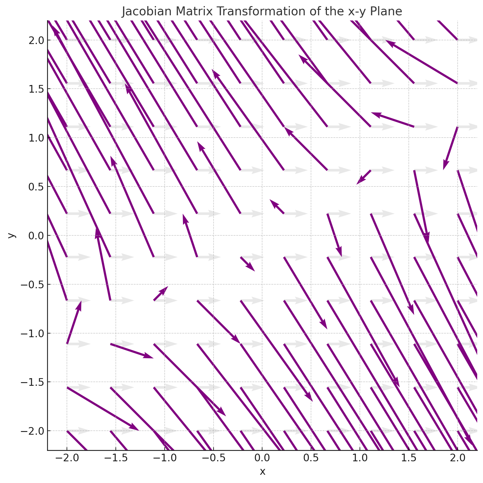
The absolute value of the determinant of the Jacobian matrix gives the factor by which the area (or volume) changes.

4. The Multivariate Change of Variables Formula

The multivariate formula is a direct extension of the 1D case. To find the joint PDF $f_{\mathbf{Y}}(\mathbf{y})$ of the transformed variables $\mathbf{Y}$, we use:
$f_{\mathbf{Y}}(\mathbf{y})=f_{\mathbf{X}}(\mathbf{h}(\mathbf{y}))\cdot \left|\det (J)\right|$
where:

• $\mathbf{x}=\mathbf{h}(\mathbf{y})$ is the inverse transformation.
• $J$ is the Jacobian matrix of the inverse transformation $\mathbf{h}$. Its elements are the partial derivatives $J_{ij}=\frac{\partial x_i}{\partial y_j}$.
• $|\det (J)|$ is the absolute value of the determinant, which is our multidimensional scaling factor.

5. A Step-by-Step Worked Example

Let's see this method in action. The process generally involves these steps:

1. Solve for the inverse transformation: Express the original variables ($X_1,X_2,\dots$) in terms of the new variables ($Y_1,Y_2,\dots$).
2. Calculate the Jacobian matrix of this inverse transformation.
3. Compute the determinant of the Jacobian matrix.
4. Substitute the inverse expressions into the original joint PDF.
5. Multiply by the absolute value of the Jacobian determinant.
6. Determine the new domain (or support) of the transformed variables. This is a critical step!

The following video provides a concise walk-through of this entire process for a two-variable transformation.

Conclusion

In this lesson, we tackled the crucial and often tricky task of transforming random variables. You now have a deep, principled understanding of why a simple substitution isn't enough and how to correctly derive the new distribution.

Key Takeaways:

• Transforming a random variable warps the underlying sample space, requiring a correction factor to ensure probability is conserved.
• In one dimension, this correction factor is the absolute value of the derivative of the inverse transformation, $|dx/dy|$.
• In multiple dimensions, this generalizes to the absolute value of the determinant of the Jacobian matrix of the inverse transformation, $|\det (J)|$.
• The procedure is systematic: find the inverse, compute the Jacobian determinant, substitute into the old PDF, multiply by the adjustment factor, and find the new domain.

Preview of the Next Lesson:
We have now explored how to define and transform specific probability distributions. But what if we don't know the exact distribution of our data? Can we still say anything useful about it? In the next lesson, we will explore Markov's and Chebyshev's inequalities, powerful tools that allow us to place bounds on probabilities even with limited information about the underlying distribution.