Markov and Chebyshev Inequalities: Proofs and Applications

Introduction

In our last lesson, we mastered the Jacobian method, a powerful tool for finding the exact probability distribution of a transformed random variable. This is invaluable when we have a complete model of our system. However, in many real-world scenarios, especially in data science, we don't have the luxury of knowing the precise distribution of our data. We might only have estimates for its mean and variance from a sample.

This raises a crucial question: can we still make meaningful probabilistic statements with such limited information? The answer is a resounding yes.

This lesson introduces two fundamental tools in probability theory: Markov's and Chebyshev's inequalities. These are known as concentration inequalities because they provide "worst-case" bounds on the probability that a random variable will deviate far from its expected value. Their power lies in their generality—they hold true for a vast range of distributions, making them indispensable in both theoretical proofs and practical data analysis.

We will derive both inequalities from first principles, explore their applications, and understand their limitations. This will directly fulfill your request for rigorous proofs coupled with intuitive understanding.

1. Markov's Inequality: Using the Mean to Bound the Tail

Let's start with the most basic inequality, which uses only the mean of a random variable.

The Intuition

Imagine you're told the average speed of cars on a highway is 60 km/h. Could 75% of the cars be traveling at 120 km/h or faster? Intuitively, this seems impossible. To maintain an average of 60, the high speeds of those cars would need to be "balanced out" by a large number of cars with very low—or even negative—speeds, which doesn't make sense in this context.

Markov's inequality formalizes this intuition. It states that if a random variable is always non-negative and has a small mean, it's unlikely to take on a very large value.

For a great visual and conceptual explanation of this "balancing" act, watch the following short clip.

Formal Statement and Proof

Markov's inequality is stated as follows:

Let $X$ be a non-negative random variable with a finite mean $\mathbb{E}[X]$. For any positive number $a>0$,
$P(X\ge a)\le \frac{\mathbb{E}[X]}{a}$

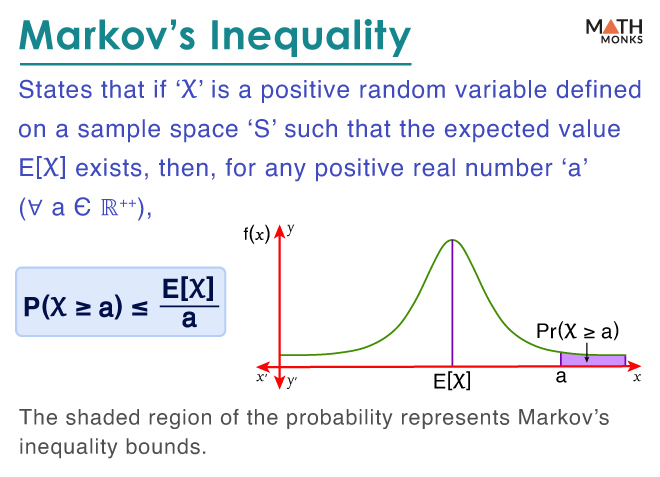
The proof is surprisingly direct and follows from the very definition of the expected value.

For your reference, here is the proof for a continuous random variable:
The expected value is defined as:
$\mathbb{E}[X]={\int }_0^{\infty }x{f}_X(x)dx(\text{since X is non-negative})$
We can split this integral at the point $a$:
$\mathbb{E}[X]={\int }_0^{a}x{f}_X(x)dx+{\int }_a^{\infty }x{f}_X(x)dx$
Since the first term ${\int }_0^{a}x{f}_X(x)dx$ is an integral of a non-negative function, it must be greater than or equal to zero. Therefore:
$\mathbb{E}[X]\ge {\int }_a^{\infty }x{f}_X(x)dx$
Within the range of this second integral ($x\ge a$), we can say that $x$ is always at least $a$. So we can replace $x$ with $a$ inside the integral, which preserves the inequality:
$\mathbb{E}[X]\ge {\int }_a^{\infty }a{f}_X(x)dx$
Factoring out the constant $a$:
$\mathbb{E}[X]\ge a{\int }_a^{\infty }{f}_X(x)dx$
The integral ${\int }_a^{\infty }{f}_X(x)dx$ is, by definition, the probability $P(X\ge a)$.
$\mathbb{E}[X]\ge a\cdot P(X\ge a)$
Rearranging for the probability gives us Markov's inequality:
$P(X\ge a)\le \frac{\mathbb{E}[X]}{a}$
This completes the proof. You can also review a written version of this proof in the "Markov's Inequality" section of this article.

2. Chebyshev's Inequality: Adding Variance for a Tighter Bound

Markov's inequality is useful, but its bound can be quite loose. It also has the strict requirement that the random variable be non-negative. We can achieve a more powerful and general result if we incorporate more information—specifically, the variance.

The Intuition

If a variable has a small variance, we know it doesn't tend to stray far from its mean. Chebyshev's inequality quantifies this. It provides a bound on the probability that a random variable deviates from its mean by more than a certain amount, and this bound depends on the variance.

Formal Statement and Proof

Let $X$ be a random variable with a finite mean $\mu$ and finite variance ${\sigma }^2$. For any positive number $k>0$,
$P(|X-\mu |\ge k\sigma )\le \frac{1}{k^2}$
This states that the probability of $X$ being $k$ or more standard deviations away from its mean is at most $1/k^2$.

The proof of Chebyshev's inequality is a brilliant application of Markov's inequality. The key insight is to apply Markov's inequality not to $X$ itself, but to a new, cleverly chosen non-negative random variable: $Y=(X-\mu {)}^2$.

1. $Y=(X-\mu {)}^2$ is always non-negative, so Markov's inequality applies to it.
2. The event $|X-\mu |\ge k\sigma$ is equivalent to the event $(X-\mu {)}^2\ge (k\sigma {)}^2$.

Watch how this plays out in the following proof.

For written proofs, you can refer to the StatLect page under the "Statement" heading or the Medium article under the "Chebyshev’s Inequality" heading. Both provide clear, step-by-step derivations.

3. Applications and Interpretation

So, when are these inequalities useful?

Their primary strength is in situations where the underlying distribution is unknown or complex.

• Engineering/Manufacturing: Suppose a manufacturing process produces resistors. You've measured that the average resistance is 100 $\Omega$ with a standard deviation of 2 $\Omega$, but you don't know if the distribution is Normal. What is the maximum possible percentage of resistors that could fall outside the tolerance range of 94 $\Omega$ to 106 $\Omega$?

  • This range is $\mu \pm 6\Omega$, which is $\mu \pm 3\sigma$.
  • Using Chebyshev's with $k=3$, we get $P(|X-100|\ge 6)\le \frac{1}{3^2}=\frac{1}{9}\approx 11.1\%$.
  • You can guarantee that at most 11.1% of your resistors will be out of spec, regardless of the shape of the distribution.

• Theoretical Importance: The most famous application of Chebyshev's inequality is in proving the Weak Law of Large Numbers (WLLN), which we will do in our next lesson. The WLLN is the theorem that gives formal justification to the practice of using a sample average to estimate a population mean.

Self-Test

To solidify your understanding, work through the examples and solved exercises on the StatLect page. This will give you practice in applying the formulas to concrete problems, which aligns with your request for practical exercises.

Conclusion

In this lesson, you've added two powerful, distribution-free inequalities to your toolkit. They allow you to make concrete probabilistic statements even with minimal information.

Key Takeaways:

• Markov's Inequality provides a loose upper bound on the probability that a non-negative random variable exceeds some value, using only its mean.
• Chebyshev's Inequality provides a tighter bound on the probability that any random variable deviates from its mean by a certain number of standard deviations, using both its mean and variance.
• The proof of Chebyshev's is a clever application of Markov's to the squared deviation from the mean, $(X-\mu {)}^2$.
• These inequalities are invaluable when the underlying probability distribution is unknown, providing worst-case guarantees.

Preview of the Next Lesson:
With Chebyshev's inequality now firmly understood, we have the primary tool needed to tackle one of the most fundamental theorems in all of statistics. In the next lesson, we will use it to formally derive the Weak Law of Large Numbers (WLLN). We will also explore the related Central Limit Theorem (CLT), explaining the profound difference between them and their implications for data science.