Orthogonal Projection and Least Squares

1. From Lines to Subspaces: The Geometry of Projection

Before we tackle the full OLS problem, let's build our geometric intuition by understanding how to project a vector onto a line, and then onto a plane (or a more general subspace). The key idea is that the shortest distance from a point to a subspace is always along the perpendicular.

The following video provides an excellent, step-by-step development of this idea. It begins with the simple projection of one vector onto another and builds up to the general formula for projecting onto a subspace spanned by a set of basis vectors.

The video demonstrates that finding the projection $\hat{\mathbf{y}}$ of a vector $\mathbf{y}$ onto the subspace spanned by the columns of a matrix $\mathbf{X}$ involves finding the point $\hat{\mathbf{y}}$ in that subspace such that the error vector $\mathbf{y}-\hat{\mathbf{y}}$ is orthogonal to the subspace.

2. The Best Approximation Theorem

The video gave us the intuition: the projection is the "closest" vector. This is a fundamental concept in linear algebra, formalized by the Best Approximation Theorem.

Let's put our OLS problem into this context:

• The vector of observations, $\mathbf{y}$, is a point in ${\mathbb{R}}^n$.
• The set of all possible predictions, $\{\mathbf{X}\mathbf{\beta }\mid \mathbf{\beta }\in {\mathbb{R}}^{p+1}\}$, forms the column space of the design matrix $\mathbf{X}$, which we denote as Col($\mathbf{X}$). This is a subspace of ${\mathbb{R}}^n$.

The OLS problem asks to find $\hat{\mathbf{\beta }}$ that minimizes $||\mathbf{y}-\mathbf{X}\mathbf{\beta }|{|}^2$. Geometrically, this means we are looking for the vector $\hat{\mathbf{y}}=\mathbf{X}\hat{\mathbf{\beta }}$ in Col($\mathbf{X}$) that is closest to $\mathbf{y}$.

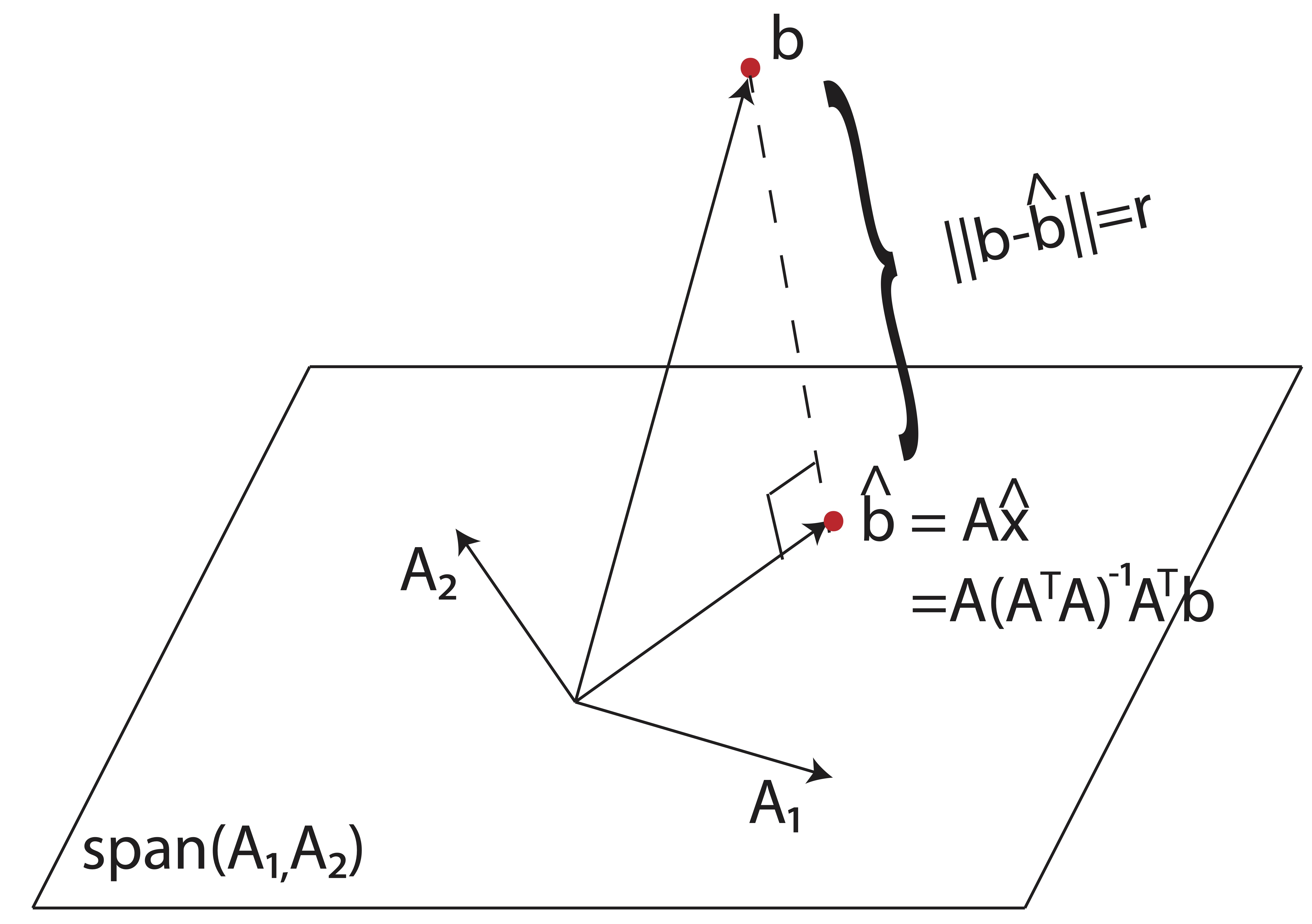
The Best Approximation Theorem guarantees that this closest vector is the orthogonal projection.

3. Deriving the Normal Equations Geometrically

Now we can connect the geometry directly to the Normal Equations we found in the last lesson.

The Best Approximation Theorem tells us that for the OLS solution $\hat{\mathbf{\beta }}$, the residual vector $\mathbf{r}=\mathbf{y}-\mathbf{X}\hat{\mathbf{\beta }}$ must be orthogonal to the subspace Col($\mathbf{X}$).

If a vector is orthogonal to a subspace, it must be orthogonal to every vector that spans that subspace. The columns of $\mathbf{X}$ are a spanning set for Col($\mathbf{X}$). Let the columns of $\mathbf{X}$ be ${\mathbf{x}}_0,{\mathbf{x}}_1,\dots ,{\mathbf{x}}_p$. Then:

In transpose notation, this is:

We can stack all of these $p+1$ equations into a single matrix equation. The rows of the matrix ${\mathbf{X}}^T$ are precisely the vectors ${\mathbf{x}}_j^T$. Therefore, the entire system of orthogonality conditions can be written as:

By distributing ${\mathbf{X}}^T$, we get:

Rearranging this gives us the Normal Equations:

This is the exact same result we derived using calculus, but this time, it emerges from a purely geometric argument based on orthogonality.

4. The Projection Matrix

Since the OLS prediction $\hat{\mathbf{y}}$ is the orthogonal projection of $\mathbf{y}$ onto Col($\mathbf{X}$), there must be a matrix that performs this projection. This is known as the projection matrix, often denoted $\mathbf{P}$ (or $\mathbf{H}$ for "hat matrix").

We know the formula for the coefficients:

And we know the predicted values are $\hat{\mathbf{y}}=\mathbf{X}\hat{\mathbf{\beta }}$. Substituting the first equation into the second gives:

The matrix in the brackets is the projection matrix:

This matrix projects any vector $\mathbf{y}\in {\mathbb{R}}^n$ onto the subspace spanned by the columns of $\mathbf{X}$.

A fun mathematical fact about projection matrices is that they are idempotent, meaning ${\mathbf{P}}^2=\mathbf{P}$. This makes perfect geometric sense: if you project a vector that is already in the subspace, it should not change. Projecting a second time does nothing new.

For a worked example of how to compute and use a projection matrix, the following video is very instructive.

Conclusion

In this lesson, we explored the beautiful geometric foundation of Ordinary Least Squares, providing a powerful alternative to the calculus-based derivation from our previous session. This new perspective allows us to understand why the OLS solution takes the form it does.

Key Takeaways:

• Minimizing the sum of squared errors is geometrically equivalent to finding the vector $\hat{\mathbf{y}}$ in the column space of $\mathbf{X}$ that is closest to the observation vector $\mathbf{y}$.
• The Best Approximation Theorem states that this closest vector is the orthogonal projection of $\mathbf{y}$ onto the column space of $\mathbf{X}$.
• The orthogonality condition—that the residual vector $\mathbf{y}-\hat{\mathbf{y}}$ is orthogonal to Col($\mathbf{X}$)—leads directly to the Normal Equations: ${\mathbf{X}}^T\mathbf{X}\hat{\mathbf{\beta }}={\mathbf{X}}^T\mathbf{y}$.
• The OLS predictions can be obtained by applying the projection matrix $\mathbf{P}=\mathbf{X}({\mathbf{X}}^T\mathbf{X}{)}^{-1}{\mathbf{X}}^T$ to the observation vector $\mathbf{y}$.

Preview of the Next Lesson:

Now that we have derived the OLS estimator from two different perspectives and understand its properties, we are ready to analyze its performance. In the next lesson, we will dive into the optimality of estimators. We will state the conditions for and derive the Cramér-Rao Lower Bound (CRLB), a fundamental limit on the variance of any unbiased estimator. Then, we will prove the famous Gauss-Markov theorem, which establishes that under certain assumptions, the OLS estimator is the Best Linear Unbiased Estimator (BLUE). This will fulfill your request for these important proofs and solidify our theoretical understanding of statistical estimation.