Matrix Calculus for OLS Normal Equations

1. Setting Up the OLS Problem

Before we can perform the calculus, we must first express the linear regression model and its associated error function in the language of linear algebra: matrix notation. This provides a compact and powerful way to handle models with any number of features.

A multiple linear regression model attempts to describe a dependent variable, $y$, as a linear combination of several independent variables or features, $x_1,x_2,\dots ,x_p$. For $n$ observations, the model for the $i$-th observation is:

Here, ${\beta }_0$ is the intercept, ${\beta }_j$ are the coefficients for each feature, and ${ϵ}_i$ is the error term.

We can represent this entire system of $n$ equations compactly as:

where:

• $\mathbf{y}$ is the $n\times 1$ vector of observed outcomes.
• $\mathbf{X}$ is the $n\times (p+1)$ design matrix, where the first column is all ones (for the intercept ${\beta }_0$) and subsequent columns contain the values of the features.
• $\mathbf{\beta }$ is the $(p+1)\times 1$ vector of unknown coefficients.
• $\mathbf{ϵ}$ is the $n\times 1$ vector of error terms.

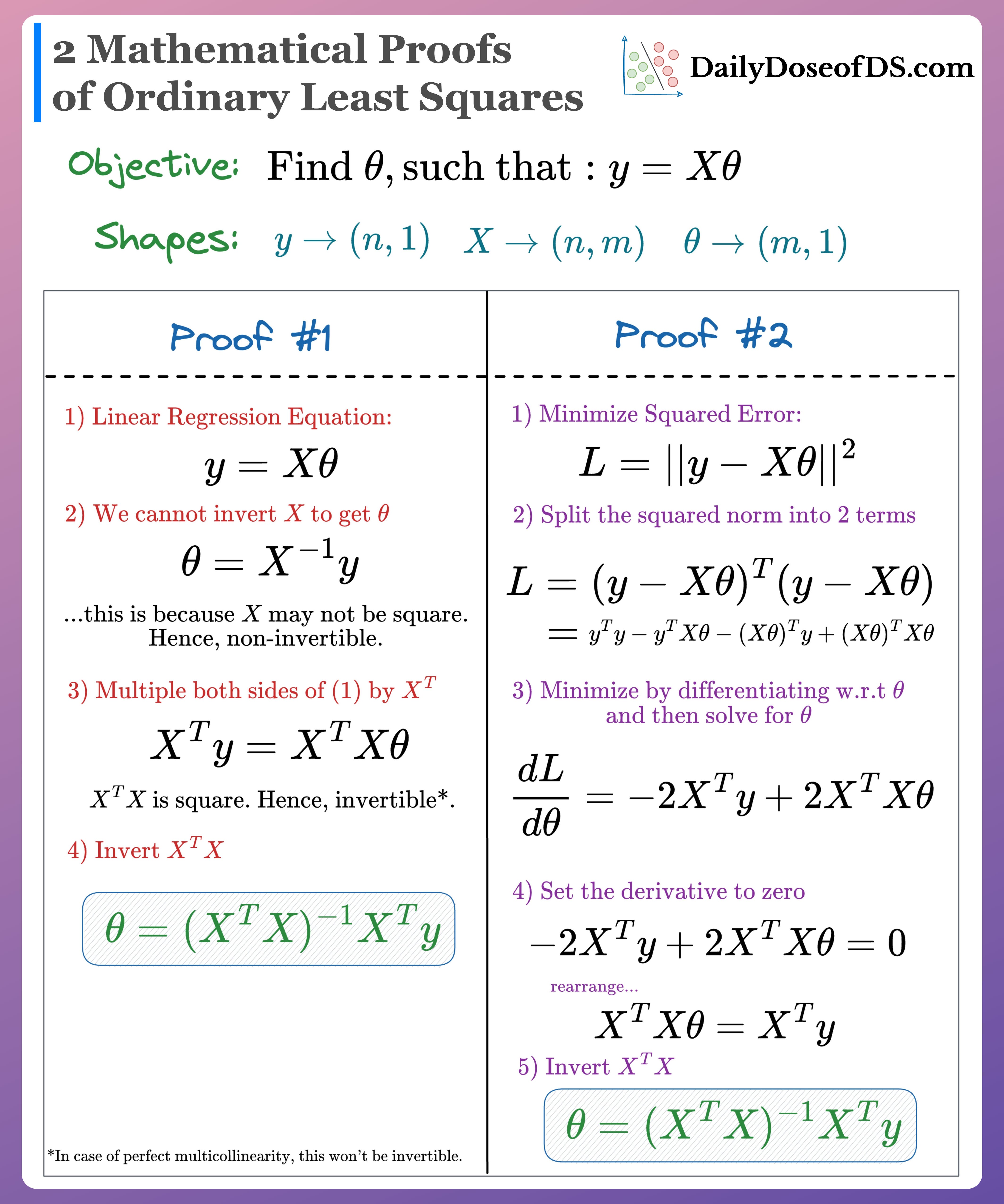
The goal of OLS is to find the coefficient vector $\hat{\mathbf{\beta }}$ that minimizes the Sum of Squared Residuals (SSR). The residual for the $i$-th observation is $r_i=y_i-{\hat{y}}_i$, where ${\hat{y}}_i$ is the predicted value. In matrix form, the vector of residuals is $\mathbf{r}=\mathbf{y}-\mathbf{X}\hat{\mathbf{\beta }}$.

The SSR, our objective function to minimize, is the squared Euclidean norm of this residual vector:

This function $J(\mathbf{\beta })$ is a scalar value representing the total squared error for a given choice of $\mathbf{\beta }$. Our task is to find the $\mathbf{\beta }$ that makes this value as small as possible.

2. Deriving the Normal Equations with Matrix Calculus

Now we come to the core of the lesson: deriving the solution by minimizing $J(\mathbf{\beta })$. This involves expanding the objective function, differentiating it with respect to the vector $\mathbf{\beta }$, setting the result to zero, and solving.

The following two short videos provide an excellent step-by-step walkthrough of this derivation.

As shown in the video, the first step is to expand the objective function:

Noting that the middle two terms are scalars and thus equal to their own transpose, we can combine them:

Next, we take the gradient (the vector of partial derivatives) with respect to $\mathbf{\beta }$ and set it to zero. The video walks through this, resulting in:

Now, let's see how to solve this for $\hat{\mathbf{\beta }}$.

Following the final steps, we rearrange the equation:

This elegant and fundamental result is known as the Normal Equation(s).

To get our final solution, we solve for $\mathbf{\beta }$ by pre-multiplying by the inverse of ${\mathbf{X}}^T\mathbf{X}$, assuming it exists:

This is the celebrated closed-form solution for Ordinary Least Squares.

3. A More Formal Calculus Approach

To reinforce your understanding and satisfy your preference for formal mathematics, let's re-derive the result using the standard rules of matrix calculus more directly.

As the reading shows, we can use two key gradient identities:

1. ${\nabla }_{\mathbf{x}}({\mathbf{c}}^T\mathbf{x})=\mathbf{c}$
2. ${\nabla }_{\mathbf{x}}({\mathbf{x}}^T\mathbf{Ax})=(\mathbf{A}+{\mathbf{A}}^T)\mathbf{x}$

Our objective function was: $J(\mathbf{\beta })={\mathbf{y}}^T\mathbf{y}-2{\mathbf{y}}^T\mathbf{X}\mathbf{\beta }+{\mathbf{\beta }}^T({\mathbf{X}}^T\mathbf{X})\mathbf{\beta }$. Let's apply the gradient ${\nabla }_{\mathbf{\beta }}$ to each term:

• ${\nabla }_{\mathbf{\beta }}({\mathbf{y}}^T\mathbf{y})=0$ (no $\mathbf{\beta }$ term)
• ${\nabla }_{\mathbf{\beta }}(-2{\mathbf{y}}^T\mathbf{X}\mathbf{\beta })=-2({\mathbf{y}}^T\mathbf{X}{)}^T=-2{\mathbf{X}}^T\mathbf{y}$ (using rule 1, where ${\mathbf{c}}^T=-2{\mathbf{y}}^T\mathbf{X}$)
• ${\nabla }_{\mathbf{\beta }}({\mathbf{\beta }}^T({\mathbf{X}}^T\mathbf{X})\mathbf{\beta })=(({\mathbf{X}}^T\mathbf{X})+({\mathbf{X}}^T\mathbf{X}{)}^T)\mathbf{\beta }=2({\mathbf{X}}^T\mathbf{X})\mathbf{\beta }$ (using rule 2, and since ${\mathbf{X}}^T\mathbf{X}$ is symmetric)

Combining these gives the same gradient we found before:

Setting this to zero yields the Normal Equations, as expected.

4. When Does the Solution Exist?

A crucial part of the final formula is the term $({\mathbf{X}}^T\mathbf{X}{)}^{-1}$. As you know from linear algebra, a matrix inverse exists only if the matrix is non-singular, or invertible.

For the matrix ${\mathbf{X}}^T\mathbf{X}$ to be invertible, the columns of the design matrix $\mathbf{X}$ must be linearly independent. In a regression context, this means there must be no perfect multicollinearity—no feature can be a perfect linear combination of other features. If this condition fails, the OLS solution is not unique, and we cannot find a single $\hat{\mathbf{\beta }}$ using this formula. This is both a mathematical necessity and a practical diagnostic to be aware of when building models.

Conclusion

In this lesson, we transitioned from the probabilistic framework of MLE to the geometric error-minimization framework of OLS. By applying matrix calculus, we derived one of the most fundamental results in statistical learning.

Key Takeaways:

• The OLS objective is to minimize the Sum of Squared Residuals (SSR), given by the objective function $J(\mathbf{\beta })=(\mathbf{y}-\mathbf{X}\mathbf{\beta }{)}^T(\mathbf{y}-\mathbf{X}\mathbf{\beta })$.
• By finding the gradient of $J(\mathbf{\beta })$ with respect to $\mathbf{\beta }$ and setting it to zero, we derive the Normal Equations: $${\mathbf{X}}^T\mathbf{X}\hat{\mathbf{\beta }}={\mathbf{X}}^T\mathbf{y}$$
• Solving the Normal Equations gives the closed-form solution for the OLS coefficient estimates: $$\hat{\mathbf{\beta }}=({\mathbf{X}}^T\mathbf{X}{)}^{-1}{\mathbf{X}}^T\mathbf{y}$$
• This solution is unique if and only if the matrix ${\mathbf{X}}^T\mathbf{X}$ is invertible, which requires the features in $\mathbf{X}$ to be linearly independent.

Preview of the Next Lesson:

While the calculus approach is powerful, it doesn't provide the full intuition. Why are the Normal Equations called "normal"? The name hints at orthogonality. In the next lesson, we will delve into the geometric interpretation of Least Squares. We will show that the OLS solution is equivalent to finding the orthogonal projection of the outcome vector $\mathbf{y}$ onto the subspace spanned by the columns of the design matrix $\mathbf{X}$. This will provide a beautiful and deeply intuitive understanding of why OLS works the way it does, connecting directly to your background in physics and vector mechanics.