NumPy for N-Dimensional Array Operations

1. Why Not Just Use Python Lists?

Before we dive into NumPy, it's essential to understand why it's the preferred library for numerical data over Python's built-in lists. While lists are flexible, they are not optimized for large-scale numerical operations. NumPy arrays offer three key advantages:

1. Speed: NumPy operations are executed by pre-compiled C code, making them significantly faster than operations on Python lists, which require slow Python loops.
2. Memory Efficiency: NumPy arrays are homogeneous (all elements are of the same type), which allows for a more compact memory layout than Python lists that need to store type information for each element.
3. Convenience: NumPy enables you to perform operations on entire arrays at once. This is called vectorization, and it allows for cleaner, more readable code without explicit loops.

To see a practical comparison, the following video provides a clear demonstration.

2. The Anatomy of a NumPy Array

The heart of NumPy is the ndarray, or N-dimensional array. It's a grid of values, all of the same type. To use it effectively, we need to understand its core attributes.

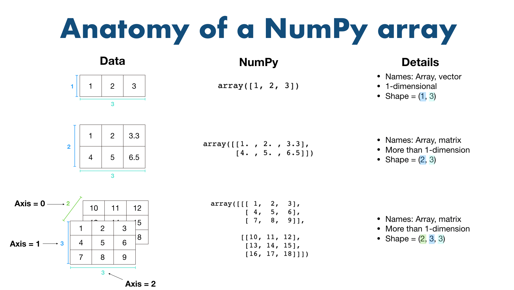
The most important attributes of an ndarray are:

• ndarray.ndim: The number of axes (dimensions) of the array.
• ndarray.shape: A tuple of integers indicating the size of the array in each dimension. For a matrix with n rows and m columns, shape will be (n, m).
• ndarray.size: The total number of elements in the array.
• ndarray.dtype: An object describing the data type of the elements (e.g., int64, float64).
• ndarray.itemsize: The size in bytes of each element.

The following quickstart guide from the official NumPy documentation provides a concise summary of these attributes.

Under the Hood: The Strided Memory Model

One of the secrets to NumPy's efficiency is how it handles data in memory. An ndarray is essentially a block of contiguous memory, and NumPy uses a concept called strides to know how to "step" through that memory to find the elements of the array.

This "view" mechanism is powerful. When you slice an array, you are typically creating a new view of the original data. Modifying the view will modify the original array. This is a critical feature that saves memory and boosts performance, but also one to be mindful of to avoid unintended side effects.

For a deeper dive into this concept, the following paper provides an excellent explanation.

3. Creating and Populating Arrays

Now let's get practical. There are many ways to create NumPy arrays, depending on your needs. The video below provides a hands-on tutorial.

Here is a summary of the most important creation functions:

4. Mathematical Operations on Arrays

This is where NumPy's power truly shines.

Vectorization: Element-wise Operations

Instead of looping through array elements, you can apply mathematical operations to the entire array at once.

import numpy as np




# Create an array
x = np.array([1, 2, 3, 4])




# Basic arithmetic
print(x + 5)    # Adds 5 to each element



# Output: [ 6  7  8  9]

print(x * 2)    # Multiplies each element by 2



# Output: [2 4 6 8]




# Operations between two arrays
y = np.array([10, 20, 30, 40])
print(y - x)



# Output: [ 9 18 27 36]

NumPy also provides a rich library of universal functions (ufuncs) that operate element-wise, such as np.sin(), np.sqrt(), and np.exp().

print(np.sqrt(x))



# Output: [1.         1.41421356 1.73205081 2.        ]

Broadcasting

Broadcasting is a powerful mechanism that allows NumPy to work with arrays of different shapes when performing arithmetic operations. Subject to certain constraints, the smaller array is "broadcast" across the larger array so that they have compatible shapes.

The simplest example is operating between an array and a scalar, as we saw with x + 5. The scalar 5 was effectively stretched into an array [5, 5, 5, 5] to match the shape of x.

A more complex example is adding a 1D array to a 2D array:

matrix = np.array([[1, 2, 3],
                   [4, 5, 6],
                   [7, 8, 9]])

vector = np.array([10, 20, 30])




# Add the vector to each row of the matrix
result = matrix + vector
print(result)



# Output:
# [[11 22 33]
#  [14 25 36]
#  [17 28 39]]

Here, vector was broadcast across the rows of matrix. Broadcasting avoids the need to create explicit copies of data, making it both memory-efficient and fast.

Linear Algebra

For linear algebra, NumPy distinguishes between element-wise multiplication (*) and matrix multiplication, which uses the @ operator or the .dot() method.

A = np.array([[1, 2], [3, 4]])
B = np.array([[5, 6], [7, 8]])




# Element-wise product
print(A * B)



# Output:
# [[ 5 12]
#  [21 32]]




# Matrix product
print(A @ B)



# Output:
# [[19 22]
#  [43 50]]

5. Accessing and Manipulating Array Data

Being able to create and operate on arrays is useful, but often you need to select, slice, and reshape your data.

Indexing and Slicing

• Indexing works similarly to Python lists for 1D arrays (arr[i]). For multi-dimensional arrays, you provide a tuple of indices: arr[row, column].
• Slicing allows you to select subarrays. For example, arr[0:2, 1:3] selects the first two rows and columns 1 and 2. Remember that slices create views, not copies.
• Boolean Indexing lets you select elements based on a condition. This is extremely powerful for filtering data.
• Fancy Indexing lets you use an array of indices to select elements.

The following video provides an excellent visual demonstration of these concepts, including a more complex example of boolean indexing.

Reshaping and Transposing

You can change an array's shape without changing its data.

• arr.reshape(new_shape) returns a new array (as a view if possible) with a different shape.
• arr.T returns the transpose of the array.
• arr.ravel() and arr.flatten() convert a multi-dimensional array into a 1D array. ravel() returns a view if possible, while flatten() always returns a copy.

6. Axis-based and Aggregate Operations

NumPy provides functions to perform calculations across the entire array or along a specific axis.

• Aggregate functions like arr.sum(), arr.mean(), arr.std(), arr.min(), and arr.max() compute a single value from the array.
• Axis-based operations allow you to perform these aggregations along a specific dimension (e.g., row-wise or column-wise). In a 2D array, axis=0 refers to columns, and axis=1 refers to rows.

matrix = np.array([[1, 2, 3],
                   [4, 5, 6]])




# Sum of all elements
print(matrix.sum())      # Output: 21




# Sum along columns (axis=0)
print(matrix.sum(axis=0))  # Output: [5 7 9]




# Sum along rows (axis=1)
print(matrix.sum(axis=1))  # Output: [ 6 15]

Self-Test and Practice

Now it's time to apply what you've learned. Try to solve the following problems using NumPy.

1. Create a 1D NumPy array containing all integers from 10 to 50.
2. Create a 5x5 matrix where the values on the border are 1 and the values inside are 0.
3. Create a 3x3 identity matrix and then find its determinant and inverse using np.linalg.det() and np.linalg.inv().
4. Generate a 10x10 array of random integers between 1 and 100.
   • Find the minimum and maximum values in the array.
   • Replace all values greater than 50 with the value 50.
   • Normalize the array: subtract the mean of the array from each element and then divide by the standard deviation.
5. Challenge: Create a 2D plot of the "sombrero" function, $z=\frac{\sin (\sqrt{x^2+y^2})}{\sqrt{x^2+y^2}}$, for x and y in the range [-10, 10].
   • Hint: Use np.linspace() to create x and y vectors. Then, use np.meshgrid() to create coordinate matrices from them. Finally, calculate z and use matplotlib.pyplot.imshow() to visualize the result. This problem combines array creation, broadcasting, and universal functions.

Conclusion

In this lesson, you've taken the first crucial step into the world of data science with Python. You've learned:

• NumPy's ndarray is the high-performance data structure for numerical data in Python.
• Vectorization and broadcasting allow for fast, efficient, and readable code by eliminating explicit loops.
• NumPy provides a comprehensive toolkit for creating, manipulating, and performing mathematical and linear algebra operations on N-dimensional arrays.
• Understanding the memory model (views vs. copies) is key to writing efficient and bug-free code.

In our next lesson, we will build directly on this foundation. We'll introduce Pandas, a library that uses NumPy arrays under the hood to provide a more powerful and intuitive object for working with labeled, tabular data—the DataFrame. This is the primary tool for data loading, cleaning, and exploratory analysis in Python.