K-means and Voronoi Diagrams

1. What is a Voronoi Tessellation?

Before we connect this concept to K-means, let's first build an intuition for what a Voronoi tessellation (or Voronoi diagram) is. You may have encountered these patterns before, as they appear frequently in physics, biology, and engineering.

To get an intuitive feel for this, let's watch a short video that illustrates how these patterns form.

As the video explained, a Voronoi tessellation is a partition of a plane into regions based on the distance to a specified set of points, often called "seeds" or "sites".

Formal Definition:
Given a set of $k$ seed points $\{{\mathbf{c}}_1,{\mathbf{c}}_2,\dots ,{\mathbf{c}}_k\}$ in a space (e.g., a 2D plane), the Voronoi cell $S_i$ corresponding to the seed ${\mathbf{c}}_i$ is the set of all points in the space that are closer to ${\mathbf{c}}_i$ than to any other seed ${\mathbf{c}}_j$.

Mathematically, the Voronoi cell $S_i$ is defined as:
$S_i=\{\mathbf{x}|\Vert \mathbf{x}-{\mathbf{c}}_i\Vert \le \Vert \mathbf{x}-{\mathbf{c}}_j\Vert \text{ for all }j\ne i\}$

The collection of all these $k$ cells is the Voronoi tessellation. The boundaries of the cells are formed by points that are equidistant to two (or more) seeds. In a 2D plane, these boundaries are straight line segments. In 3D space, they are planes. In higher dimensions, they are hyperplanes.

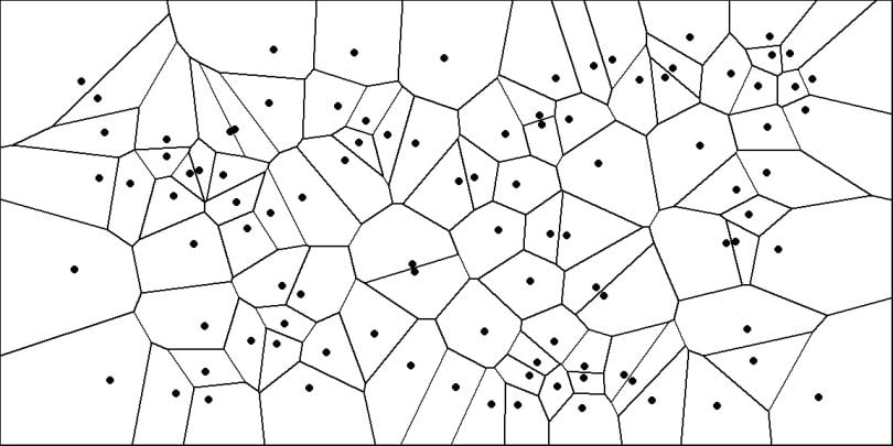
2. The Connection Between K-means and Voronoi Tessellations

Now, let's revisit the K-means algorithm. Do you see the connection?

The assignment step of the K-means algorithm, which we derived in the last lesson, states:

Assign each data point ${\mathbf{x}}^{(n)}$ to the cluster corresponding to the nearest centroid.

If we consider the cluster centroids $\{{\mathbf{\mu }}_1,\dots ,{\mathbf{\mu }}_K\}$ as the "seeds" of a Voronoi diagram, then the assignment step does nothing more than determine which Voronoi cell each data point falls into.

• The K-means centroids ${\mathbf{\mu }}_k$ are the seeds of the Voronoi tessellation.
• Each K-means cluster ${\hat{C}}_k$ is simply the set of data points that lie within the Voronoi cell $S_k$.

This is the core geometric intuition of K-means. The algorithm partitions the entire feature space into a Voronoi diagram defined by the centroids, and each partition becomes a cluster.

The following reading makes this connection explicit and provides excellent visualizations.

Another excellent resource confirms this interpretation.

3. The Iterative Process, Viewed Geometrically

We can now re-frame the entire K-means algorithm in geometric terms:

1. Initialization: Place $K$ centroids (seeds) in the space.
2. Assignment Step: Construct the Voronoi tessellation based on the current centroid locations. All data points within a single Voronoi cell form a cluster.
3. Update Step: For each cell, calculate the center of mass (mean) of all the data points it contains. Move the centroid to this new position.
4. Repeat: Go back to step 2. Since the centroids have moved, the Voronoi tessellation will change. Repeat this process until the centroids no longer move significantly, at which point the tessellation becomes stable.

The visualizations in the "Visualization" section of the blog post by Antoine Broyelle perfectly illustrate this dynamic process of the Voronoi cells shifting and reshaping as the centroids are updated in each iteration.

This concept extends to any number of dimensions. Your mechanical engineering background involves thinking about 3D spaces, and K-means behaves identically there, partitioning 3D space into polyhedral cells.

4. A Key Implication: Convexity

This geometric view immediately reveals a fundamental property and limitation of K-means. Voronoi cells are always convex.

A set is convex if for any two points within the set, the straight line segment connecting them is also entirely contained within the set. Because the cells are defined by linear boundaries (hyperplanes), they can never be concave or form shapes like rings or crescent moons.

Since K-means clusters are Voronoi cells, K-means can only produce convex clusters. This explains why the algorithm performs well on spherical, well-separated data but fails on datasets with more complex structures.

5. Practical Visualization with Python

To solidify this concept, you can generate and visualize Voronoi diagrams yourself using Python's scipy library. The scipy.spatial.Voronoi class takes a set of points (our centroids) and calculates the vertices and regions of the tessellation, which you can then plot with matplotlib.

Here's a quick example to demonstrate the core idea.

import numpy as np
import matplotlib.pyplot as plt
from scipy.spatial import Voronoi, voronoi_plot_2d




# Generate some random points (our 'seeds' or 'centroids')
np.random.seed(42)
points = np.random.rand(10, 2) # 10 points in 2D




# Compute Voronoi tessellation
vor = Voronoi(points)




# Plot it
fig = voronoi_plot_2d(vor)




# Add our original points
plt.plot(points[:, 0], points[:, 1], 'ro')
plt.title('Voronoi Diagram')
plt.xlabel('X-axis')
plt.ylabel('Y-axis')
plt.show()

You could extend this by first running K-means on a dataset, extracting the final centroids, and then feeding those centroids into the Voronoi function to see the final partition of the space. This exercise directly connects the algorithm's output to its geometric meaning.

Conclusion

In this lesson, we moved beyond the procedural steps of K-means to understand its inherent geometry. This perspective is crucial for developing a deep intuition for how the algorithm behaves.

Key Takeaways:

• The K-means assignment step is geometrically equivalent to partitioning the feature space into a Voronoi tessellation.
• The cluster centroids act as the seeds for the Voronoi diagram.
• The clusters themselves are the sets of data points that fall within each Voronoi cell.
• The iterative nature of K-means can be seen as a process of repeatedly recalculating the Voronoi tessellation as the centroids move to the center of mass of their respective cells.
• This geometric structure implies that K-means clusters are always convex, which explains its limitations when dealing with non-globular data shapes.

Preview of the Next Lesson

We have now established that K-means creates hard, convex partitions. But what if we want to model clusters that overlap, or where a data point could belong to multiple clusters with some probability?

In our next lesson, we will introduce the Gaussian Mixture Model (GMM). Instead of hard boundaries, GMMs use a probabilistic approach, modeling clusters as Gaussian distributions. We will derive the Expectation-Maximization (E-M) algorithm, which is used to fit GMMs, and see how it provides a "soft" alternative to the "hard" clustering of K-means.