K-Means Algorithm: Derivation and Convergence Proof

1. The K-means Objective Function

The goal of K-means is to partition a set of $N$ data points $\{{\mathbf{x}}^{(1)},\dots ,{\mathbf{x}}^{(N)}\}$ into $K$ distinct clusters. The core idea is to find clusters where the data points within each cluster are as similar as possible. In K-means, "similarity" is defined by spatial proximity. We want to minimize the intra-cluster variance, which is equivalent to minimizing the sum of squared Euclidean distances from each data point to the center of its assigned cluster.

Let's formalize this. We need to find:

1. A set of $K$ cluster centroids (or means), $\{{\mathbf{\mu }}_1,{\mathbf{\mu }}_2,\dots ,{\mathbf{\mu }}_K\}$.
2. An assignment of each data point ${\mathbf{x}}^{(n)}$ to one of these clusters.

We can define an objective function, often denoted $\hat{\mathcal{J}}$, which we aim to minimize. This function is the sum of the squared distances between each data point and the centroid of the cluster it's assigned to.

As defined in the reading, our objective is to minimize:
$\hat{\mathcal{J}}={\sum }_{k=1}^K{\sum }_{{\mathbf{x}}^{(n)}\in {\hat{C}}_k}{\Vert {\mathbf{x}}^{(n)}-{\mathbf{\mu }}_k\Vert }^2$
where ${\hat{C}}_k$ is the set of points assigned to cluster $k$, and ${\mathbf{\mu }}_k$ is the centroid of that cluster. We want to find the cluster assignments and centroid locations that make this total "cost" as small as possible.

2. Deriving the K-means Algorithm

Finding the global minimum of $\hat{\mathcal{J}}$ is an NP-hard problem. This means we can't solve it directly for any reasonably sized dataset. Instead, K-means uses an iterative, greedy approach often called alternating optimization or coordinate descent. We don't optimize for cluster assignments and centroids simultaneously. Instead, we alternate between two steps:

1. Assignment Step: Assume the centroids are fixed, and find the optimal assignment for each data point.
2. Update Step: Assume the assignments are fixed, and find the new optimal locations for the centroids.

Let's derive the rules for each step.

Derivation of the Assignment Step

Assume we have a fixed set of centroids $\{{\mathbf{\mu }}_1,\dots ,{\mathbf{\mu }}_K\}$ from the previous iteration. We need to assign each data point ${\mathbf{x}}^{(n)}$ to a cluster. Our goal is to minimize the total cost $\hat{\mathcal{J}}$.

The total cost is a sum of individual costs for each point: ${\sum }_{n=1}^N{\Vert {\mathbf{x}}^{(n)}-{\mathbf{\mu }}_{\text{assigned}}\Vert }^2$. To minimize this sum, we can simply minimize each term independently. For a single data point ${\mathbf{x}}^{(n)}$, its contribution to the cost is minimized by assigning it to the cluster $k$ whose centroid ${\mathbf{\mu }}_k$ is the closest.

This gives us our first rule:
Assignment Rule: Assign each data point ${\mathbf{x}}^{(n)}$ to the cluster corresponding to the nearest centroid.
${\hat{y}}^{(n)}=\underset{k\in \{1,\dots ,K\}}{\mathrm{argmin}}{\Vert {\mathbf{x}}^{(n)}-{\mathbf{\mu }}_k\Vert }^2$
Here, ${\hat{y}}^{(n)}$ is the cluster index assigned to point ${\mathbf{x}}^{(n)}$.

Derivation of the Update Step

Now, assume we have fixed cluster assignments from the previous step. For each cluster $k$, we have a set of points ${\hat{C}}_k$. We need to find the new location for the centroid ${\mathbf{\mu }}_k$ that minimizes the sum of squared distances for just that cluster.

The cost for a single cluster $k$ is:
${\hat{\mathcal{J}}}_k({\mathbf{\mu }}_k)={\sum }_{{\mathbf{x}}^{(n)}\in {\hat{C}}_k}{\Vert {\mathbf{x}}^{(n)}-{\mathbf{\mu }}_k\Vert }^2$
This is a quadratic function of ${\mathbf{\mu }}_k$ and is therefore convex. We can find the minimum by taking the gradient with respect to ${\mathbf{\mu }}_k$ and setting it to zero. Your background in mechanics and vector calculus will be useful here.

Let's expand the squared norm: ${\Vert \mathbf{a}\Vert }^2={\mathbf{a}}^T\mathbf{a}$.
${\hat{\mathcal{J}}}_k({\mathbf{\mu }}_k)={\sum }_{{\mathbf{x}}^{(n)}\in {\hat{C}}_k}({\mathbf{x}}^{(n)}-{\mathbf{\mu }}_k{)}^T({\mathbf{x}}^{(n)}-{\mathbf{\mu }}_k)$
The gradient with respect to the vector ${\mathbf{\mu }}_k$ is:
${\nabla }_{{\mathbf{\mu }}_k}{\hat{\mathcal{J}}}_k({\mathbf{\mu }}_k)={\sum }_{{\mathbf{x}}^{(n)}\in {\hat{C}}_k}{\nabla }_{{\mathbf{\mu }}_k}\left(({\mathbf{x}}^{(n)}{)}^T{\mathbf{x}}^{(n)}-2({\mathbf{x}}^{(n)}{)}^T{\mathbf{\mu }}_k+{\mathbf{\mu }}_k^T{\mathbf{\mu }}_k\right)$
Using the standard identities ${\nabla }_{\mathbf{v}}({\mathbf{a}}^T\mathbf{v})=\mathbf{a}$ and ${\nabla }_{\mathbf{v}}({\mathbf{v}}^T\mathbf{v})=2\mathbf{v}$, we get:
${\nabla }_{{\mathbf{\mu }}_k}{\hat{\mathcal{J}}}_k({\mathbf{\mu }}_k)={\sum }_{{\mathbf{x}}^{(n)}\in {\hat{C}}_k}(-2{\mathbf{x}}^{(n)}+2{\mathbf{\mu }}_k)=-2{\sum }_{{\mathbf{x}}^{(n)}\in {\hat{C}}_k}({\mathbf{x}}^{(n)}-{\mathbf{\mu }}_k)$
Setting the gradient to zero to find the minimum:
$-2{\sum }_{{\mathbf{x}}^{(n)}\in {\hat{C}}_k}({\mathbf{x}}^{(n)}-{\mathbf{\mu }}_k)=0$
${\sum }_{{\mathbf{x}}^{(n)}\in {\hat{C}}_k}{\mathbf{x}}^{(n)}-{\sum }_{{\mathbf{x}}^{(n)}\in {\hat{C}}_k}{\mathbf{\mu }}_k=0$
Let $N_k=|{\hat{C}}_k|$ be the number of points in cluster $k$.
${\sum }_{{\mathbf{x}}^{(n)}\in {\hat{C}}_k}{\mathbf{x}}^{(n)}-N_k{\mathbf{\mu }}_k=0$
${\mathbf{\mu }}_k=\frac{1}{N_k}{\sum }_{{\mathbf{x}}^{(n)}\in {\hat{C}}_k}{\mathbf{x}}^{(n)}$

This elegant result gives us our second rule:
Update Rule: The optimal centroid for a cluster is the mean (or center of mass) of all the data points assigned to it.

The following resource provides a formal write-up of these two derivations.

Visually, this iterative process of assigning points and updating centroids looks like this:

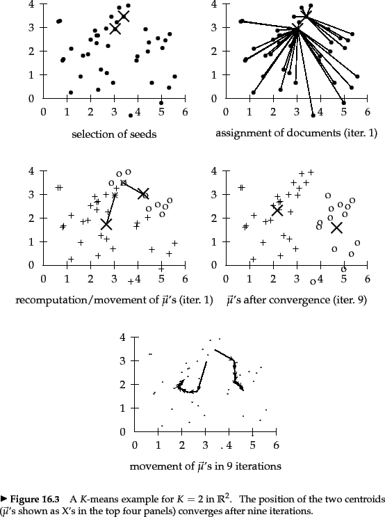
3. Proof of Convergence

We've derived the steps of the algorithm, but how do we know it will ever stop? We need to prove that it converges. The proof is surprisingly straightforward and relies on two key facts.

1. The objective function $\hat{\mathcal{J}}$ is monotonically non-increasing at every step.
2. The number of possible partitions of the data is finite.

Let's watch a video that walks through the argument for convergence in detail.

Let's summarize the proof formally. Let ${\hat{\mathcal{J}}}^{(t)}$ be the value of the objective function at the beginning of iteration $t$. The centroids are ${\mathbf{\mu }}^{(t)}$ and the cluster assignments are ${\hat{C}}^{(t)}$.

1. Assignment Step: We re-assign points to their closest centroid in ${\mathbf{\mu }}^{(t)}$ to get new clusters ${\hat{C}}^{(t+1)}$. By the definition of this step (assigning each point to its closest centroid), the sum of squared distances cannot increase. If any point moves to a new cluster, it must be because its new centroid is strictly closer, so the cost will strictly decrease.
   $\hat{\mathcal{J}}({\hat{C}}^{(t+1)},{\mathbf{\mu }}^{(t)})\le \hat{\mathcal{J}}({\hat{C}}^{(t)},{\mathbf{\mu }}^{(t)})$

2. Update Step: We compute the new centroids ${\mathbf{\mu }}^{(t+1)}$ by taking the mean of the points in the new clusters ${\hat{C}}^{(t+1)}$. As we proved in our derivation of the update step (and as shown in the video's "Fact 1"), the mean is the point that minimizes the sum of squared distances for a set of points. Therefore, this step also cannot increase the cost.
   $\hat{\mathcal{J}}({\hat{C}}^{(t+1)},{\mathbf{\mu }}^{(t+1)})\le \hat{\mathcal{J}}({\hat{C}}^{(t+1)},{\mathbf{\mu }}^{(t)})$

Combining these two inequalities, we get:
${\hat{\mathcal{J}}}^{(t+1)}=\hat{\mathcal{J}}({\hat{C}}^{(t+1)},{\mathbf{\mu }}^{(t+1)})\le \hat{\mathcal{J}}({\hat{C}}^{(t+1)},{\mathbf{\mu }}^{(t)})\le \hat{\mathcal{J}}({\hat{C}}^{(t)},{\mathbf{\mu }}^{(t)})={\hat{\mathcal{J}}}^{(t)}$
This shows that the objective function is monotonically non-increasing.

Since the objective function $\hat{\mathcal{J}}$ can never be negative, it is bounded below by 0. Furthermore, there is a finite number of ways to partition $N$ data points into $K$ clusters (the number is at most $K^N$). Since the cost function strictly decreases whenever the cluster assignments change, the algorithm can never repeat a partition. A sequence that is monotonically decreasing and bounded below, and can only take on a finite number of values, must converge.

Therefore, the K-means algorithm is guaranteed to converge to a local minimum in a finite number of steps. It's important to note that it does not guarantee finding the global minimum; the final result depends on the initial placement of centroids.

Conclusion

In this lesson, we have rigorously analyzed the K-means algorithm. We treated it not just as a set of instructions, but as an optimization procedure for a clearly defined objective function.

Key Takeaways:

• K-means aims to minimize the sum of squared Euclidean distances from each point to its assigned cluster centroid.
• The algorithm proceeds via alternating optimization:
  1. Assignment Step: Each point is assigned to its closest centroid.
  2. Update Step: Each centroid is moved to the mean of the points assigned to it.
• Both of these steps were derived by minimizing the objective function while holding the other variable fixed.
• Convergence is guaranteed because the objective function monotonically decreases at each step, and there is a finite number of possible cluster configurations. The algorithm stops when cluster assignments no longer change, which corresponds to a local minimum of the cost function.

Preview of the Next Lesson

We've established how K-means works and that it converges. However, K-means makes a "hard" assignment—each point belongs to exactly one cluster. What if we want to model "soft" assignments, where a point might belong to multiple clusters with varying probabilities? In our next lesson, we will explore the Gaussian Mixture Model (GMM), which provides this probabilistic perspective on clustering. We will derive its Expectation-Maximization (E-M) algorithm and compare its assumptions and use cases to those of K-means. We will also explore the beautiful geometric interpretation of K-means as creating a Voronoi tessellation of the data space.