MAP Estimation: Mode of the Posterior

1. Why Go Beyond Maximum Likelihood? The Case for Priors

Before diving into the math, it's crucial to understand why we need an alternative to Maximum Likelihood Estimation (MLE). MLE is powerful, but it can be brittle, especially with limited data. The following video provides an excellent, intuitive example of this weakness and introduces the Bayesian approach as a solution.

As the video explains, MLE only considers the likelihood $p(D|\theta )$, the probability of the data given the parameters. The core idea of Bayesian inference, and specifically MAP estimation, is to also consider our prior belief about the parameters, $p(\theta )$. We combine these two pieces of information to form the posterior distribution, $p(\theta |D)$, which represents our updated belief.

The entire MAP estimation process can be visualized with the following flowchart.

2. Deriving the MAP Estimator

Now, let's formalize this intuition. The MAP estimator is, by definition, the value of $\theta$ that maximizes the posterior probability density (or mass) function.

${\hat{\theta }}_{\text{MAP}}=\arg {\max }_{\theta }p(\theta |D)$

Using Bayes' theorem, we can rewrite the posterior:

$p(\theta |D)=\frac{p(D|\theta )p(\theta )}{p(D)}$

So, our maximization problem becomes:

${\hat{\theta }}_{\text{MAP}}=\arg {\max }_{\theta }\left[\frac{p(D|\theta )p(\theta )}{p(D)}\right]$

Here comes a crucial insight. The denominator, $p(D)=\int p(D|\theta )p(\theta )d\theta$, is the probability of the data, often called the evidence or marginal likelihood. While essential for calculating the posterior's exact value, it does not depend on $\theta$. Since we are optimizing with respect to $\theta$, $p(D)$ is just a positive constant. A constant multiplier does not change the location of the maximum. Therefore, we can drop it from the optimization problem:

${\hat{\theta }}_{\text{MAP}}=\arg {\max }_{\theta }\left[p(D|\theta )p(\theta )\right]$

This elegant result shows that the MAP estimate is found by maximizing the product of the likelihood and the prior.

The Log-Posterior Trick

As with MLE, working with products of probabilities can be numerically unstable and analytically difficult. It's almost always easier to work with their logarithms. Since the logarithm is a strictly monotonically increasing function, maximizing a function is equivalent to maximizing its logarithm.

Applying the logarithm to our objective function gives:

${\hat{\theta }}_{\text{MAP}}=\arg {\max }_{\theta }\left[\log (p(D|\theta ))+\log (p(\theta ))\right]$

This is the most common and practical form for deriving MAP estimators. It beautifully illustrates the core concept: the MAP objective is the log-likelihood (the MLE objective) plus a term representing our log-prior belief.

The following reading provides a concise summary of this derivation.

3. A Concrete Example: Estimating Coin Bias

Let's solidify the theory by deriving the MAP estimator for a classic problem: estimating the bias $\theta$ of a coin. Your background in mechanical engineering often involves modeling systems with unknown parameters; this is a direct statistical analogue.

• Likelihood Model: Let's say we have $n$ independent coin flips, resulting in $k$ heads and $n-k$ tails. The number of heads follows a Binomial distribution, so the likelihood of the data given $\theta$ is:
  $p(D|\theta )=(\genfrac{}{}{0ex}{}{n}{k}){\theta }^k(1-\theta {)}^{n-k}$

• Prior Model: We need a prior distribution for $\theta$, which represents the probability of heads. Since $\theta$ must be between 0 and 1, a natural and mathematically convenient choice is the Beta distribution, $\text{Beta}(\alpha ,\beta )$. Its PDF is:
  $p(\theta )=\frac{\Gamma (\alpha +\beta )}{\Gamma (\alpha )\Gamma (\beta )}{\theta }^{\alpha -1}(1-\theta {)}^{\beta -1}$
  The parameters $\alpha$ and $\beta$ are called hyperparameters and shape our prior belief. A higher $\alpha$ relative to $\beta$ suggests a prior belief that the coin is biased towards heads, and vice-versa.

Now, let's find the MAP estimate. We'll use the log-posterior form:

${\hat{\theta }}_{\text{MAP}}=\arg {\max }_{\theta }\left[\log (p(D|\theta ))+\log (p(\theta ))\right]$

Taking the logarithm and dropping all constants that don't depend on $\theta$:
$\log p(\theta |D)\propto \log ({\theta }^k(1-\theta {)}^{n-k})+\log ({\theta }^{\alpha -1}(1-\theta {)}^{\beta -1})$
$\log p(\theta |D)\propto k\log \theta +(n-k)\log (1-\theta )+(\alpha -1)\log \theta +(\beta -1)\log (1-\theta )$
$\log p(\theta |D)\propto (k+\alpha -1)\log \theta +(n-k+\beta -1)\log (1-\theta )$

To find the maximum, we take the derivative with respect to $\theta$ and set it to zero:
$\frac{d}{d\theta }\left[\dots \right]=\frac{k+\alpha -1}{\theta }-\frac{n-k+\beta -1}{1-\theta }=0$
Solving for $\theta$ gives our MAP estimate:
${\hat{\theta }}_{\text{MAP}}=\frac{k+\alpha -1}{n+\alpha +\beta -2}$

This derivation is a cornerstone of Bayesian estimation. The following resource provides a detailed walkthrough with excellent intuition.

4. Interpreting the MAP Estimate

Let's analyze our result for the coin bias:
${\hat{\theta }}_{\text{MAP}}=\frac{k+\alpha -1}{n+\alpha +\beta -2}$
Compare this to the MLE for the same problem, which is simply ${\hat{\theta }}_{\text{MLE}}=\frac{k}{n}$.

The MAP estimate has a beautiful interpretation: it's as if we started with $\alpha -1$ "pseudo-heads" and $\beta -1$ "pseudo-tails" from our prior belief, and then simply added the real heads ($k$) and tails ($n-k$) we observed. The final estimate is the updated proportion. The strength of our prior is controlled by the magnitude of $\alpha$ and $\beta$.

What if our prior is "uninformative"?

Consider a uniform prior, where we believe all values of $\theta$ from 0 to 1 are equally likely. This corresponds to a $\text{Beta}(1,1)$ distribution. If we set $\alpha =1$ and $\beta =1$ in our MAP formula:

${\hat{\theta }}_{\text{MAP}}=\frac{k+1-1}{n+1+1-2}=\frac{k}{n}={\hat{\theta }}_{\text{MLE}}$
This shows that MLE is a special case of MAP estimation when using a uniform prior.

The Role of Data

As the amount of data $n$ increases, the observed counts $k$ and $n-k$ will dominate the fixed prior pseudo-counts $\alpha -1$ and $\beta -1$. In the limit as $n\to \infty$, the MAP estimate converges to the MLE estimate. This makes sense: with enough evidence, our initial prior belief becomes less and less relevant.

The final segments of the videos we've used reinforce these important connections.

Conclusion

In this lesson, we have formally defined and derived the Maximum A Posteriori (MAP) estimator. We've seen how it provides a powerful framework for incorporating prior knowledge into parameter estimation, making our models more robust and intuitive.

Key Takeaways:

• The MAP estimator is the mode of the posterior distribution, representing the single most probable value for a parameter given the data.
• It is found by maximizing the product of the likelihood and the prior: ${\hat{\theta }}_{\text{MAP}}=\arg {\max }_{\theta }\left[p(D|\theta )p(\theta )\right]$.
• In practice, we maximize the sum of the log-likelihood and the log-prior: ${\hat{\theta }}_{\text{MAP}}=\arg {\max }_{\theta }\left[\log p(D|\theta )+\log p(\theta )\right]$.
• MAP estimation elegantly combines evidence from data with prior beliefs, with the prior's influence diminishing as more data becomes available.
• Maximum Likelihood Estimation (MLE) is a special case of MAP estimation that assumes a uniform (uninformative) prior.

Preview of the Next Lesson:

The final form of the MAP objective, $\arg {\max }_{\theta }\left[\log p(D|\theta )+\log p(\theta )\right]$, holds a deep connection to a concept you may have encountered in machine learning: regularization.

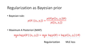
In our next lesson, we will make this connection explicit. We will formally prove that MAP estimation with a Gaussian prior on the model parameters is mathematically equivalent to performing a Least Squares regression with L2 regularization (Ridge Regression). This will bridge the gap between the Bayesian and Frequentist perspectives on model fitting.