MMSE Estimator as Posterior Mean

1. From Posterior Distributions to Point Estimates

We have a posterior distribution, which is great, but how do we choose a single value from it? Consider the posterior distribution shown below. What single point best represents it?

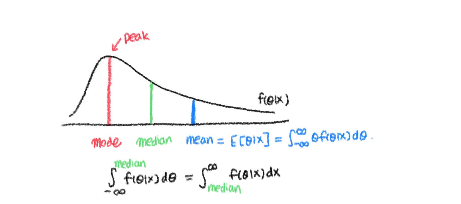
As the image suggests, there are several candidates (mean, median, mode). The "best" choice depends on how we define and penalize error. Today, we focus on a widely used and powerful criterion: the Mean Squared Error (MSE).

The MSE of an estimator $\hat{\theta }$ is defined as the expected squared difference between the estimator and the true value of the parameter $\theta$:
$\text{MSE}(\hat{\theta })=E\left[(\theta -\hat{\theta }{)}^2\right]$
Here, the expectation is taken over both the data $D$ (which makes $\hat{\theta }=g(D)$ random) and the parameter $\theta$ (which is a random variable in the Bayesian framework).

Using squared error is common in many fields of engineering and science. It penalizes large errors much more heavily than small ones, which is often a desirable property. Our goal is to find the estimator $\hat{\theta }$ that makes this value as small as possible. This is the Minimum Mean Square Error (MMSE) estimator.

2. Deriving the MMSE Estimator

We want to find the estimator, which is a function of our data $D$, let's call it $g(D)$, that minimizes the MSE.

The key to this derivation is the Law of Total Expectation, which allows us to break down the expectation into manageable parts. We can write the overall expectation as an expectation over the data $D$, of the conditional expectation of the error given the data:
$E\left[(\theta -g(D){)}^2\right]=E_D\left[E_{\theta |D}\left[(\theta -g(D){)}^2\mid D\right]\right]$
To minimize the overall expression, we can focus on minimizing the inner conditional expectation for every possible observed dataset $d$:
${\min }_{g(d)}{E}_{\theta |D}\left[(\theta -g(d){)}^2\mid D=d\right]$
Let's expand the term inside the conditional expectation. For a given $d$, $g(d)$ is just a constant value.
$E\left[(\theta -g(d){)}^2\mid D=d\right]=E[{\theta }^2-2\theta g(d)+g(d{)}^2\mid D=d]$
Using the linearity of expectation, this becomes:
$E[{\theta }^2\mid D=d]-2g(d)E[\theta \mid D=d]+g(d{)}^2$
This expression is a simple quadratic in $g(d)$. To find the value of $g(d)$ that minimizes it, we can take the derivative with respect to $g(d)$ and set it to zero, a standard optimization technique you'll be familiar with from calculus.
$\frac{\partial }{\partial g(d)}\left(E[{\theta }^2\mid D=d]-2g(d)E[\theta \mid D=d]+g(d{)}^2\right)=-2E[\theta \mid D=d]+2g(d)$
Setting this to zero gives the solution:
$-2E[\theta \mid D=d]+2g(d)=0⟹g(d)=E[\theta \mid D=d]$
The second derivative is $+2$, which is positive, confirming this is a minimum.

This is a profound result. It states that for any given data $D=d$, the estimate that minimizes the squared error is the conditional expectation of $\theta$ given the data. Therefore, the MMSE estimator is:
${\hat{\theta }}_{\text{MMSE}}(D)=E[\theta \mid D]$

This is exactly the mean of the posterior distribution $p(\theta |D)$!

The following PDF provides a formal write-up of this proof.

3. A Comprehensive Video Walkthrough

Now that you have seen the derivation from first principles, let's watch a video that ties all these concepts together. It re-derives the result using a slightly different but equivalent algebraic method ("completing the square") and discusses several important properties of the MMSE estimator.

4. Properties of the MMSE Estimator

As mentioned in the video, the MMSE estimator has several elegant properties that are worth highlighting.

Unbiasedness

The MMSE estimator is unbiased in the Bayesian sense. This means that, on average, the estimation error is zero.
$E[\text{error}]=E[\theta -{\hat{\theta }}_{\text{MMSE}}]=0$
The proof is a simple application of the law of total expectation:
$E[\theta -{\hat{\theta }}_{\text{MMSE}}]=E[E[\theta -E[\theta |D]|D]]=E[E[\theta |D]-E[\theta |D]]=E[0]=0$

The Orthogonality Principle

This is a particularly important property with a nice geometric interpretation. The estimation error of the MMSE estimator is orthogonal to any function $h(D)$ of the observations. Mathematically:
$E[(\theta -{\hat{\theta }}_{\text{MMSE}})\cdot h(D)]=0$
This is analogous to vector projections in linear algebra. The MMSE estimator $E[\theta |D]$ can be seen as the projection of the random variable $\theta$ onto the space of all possible functions of the data $D$. The error vector $(\theta -{\hat{\theta }}_{\text{MMSE}})$ is therefore orthogonal (perpendicular) to that space. This principle is fundamental in signal processing and is the basis for deriving the famous Kalman filter.

5. Example: MMSE for the Gaussian-Gaussian Model

Let's bring this back to the example from our last lesson. We were estimating the mean $\mu$ of a Gaussian, and we derived the posterior distribution to be another Gaussian:
$p(\mu |D)=\mathcal{N}(\mu |{\mu }_N,{\sigma }_N^2)$
We've just proven that the MMSE estimate is the mean of this posterior distribution. For a Gaussian $\mathcal{N}({\mu }_N,{\sigma }_N^2)$, the mean is simply ${\mu }_N$.

Therefore, the MMSE estimator for the mean of a Gaussian with a conjugate Gaussian prior is:
${\hat{\mu }}_{\text{MMSE}}=E[\mu |D]={\mu }_N={\sigma }_N^2\left(\frac{N\bar{x}}{{\sigma }^2}+\frac{{\mu }_0}{{\sigma }_0^2}\right)$
This confirms the beautiful intuition from our last lesson: the "best" estimate in a mean-squared-error sense is the precision-weighted average of our prior belief and the evidence from the data.

Conclusion

In this lesson, we established a formal procedure for obtaining a single point estimate from a full posterior distribution.

Key Takeaways:

• Point estimation aims to provide a single "best guess" for an unknown parameter based on data.
• The choice of "best" depends on the cost function used to penalize errors.
• Minimizing the Mean Squared Error (MSE), $E[(\theta -\hat{\theta }{)}^2]$, is a common and powerful choice.
• We formally derived that the estimator that minimizes the MSE is the conditional expectation of the parameter given the data, ${\hat{\theta }}_{MMSE}=E[\theta |D]$.
• Crucially, this conditional expectation is precisely the mean of the posterior distribution, $p(\theta |D)$.

Preview of the Next Lesson:

We have now seen that the mean of the posterior gives us the MMSE estimate. What about the mode? In the next lesson, we will formally define the Maximum A Posteriori (MAP) estimator, which corresponds to the mode of the posterior distribution. We will derive it, explore its properties, and uncover its fascinating and practical connection to Maximum Likelihood Estimation (MLE) and L2 regularization (Ridge Regression), bridging our Bayesian journey back to the frequentist concepts we've already mastered.