Welcome back. In our previous lessons, we analyzed the static structure of vee networks, quantifying the hinge's brokerage power with betweenness centrality and their structural autonomy using network constraint. We established that the hinge's position, bridging a structural hole, grants them significant power and freedom compared to their partners.
However, networks are more than just static wiring diagrams; they are conduits for the flow of information, emotions, and behaviors. This lesson shifts our focus from static positions to dynamic processes. We will describe common models of influence propagation in networks, such as the linear threshold and independent cascade models. These models provide the formal machinery to simulate how an idea, a new relationship norm, or even a feeling might spread through a vee. Understanding these dynamics is crucial for moving from analyzing what a network looks like to predicting what a network does.
Modeling How Influence Spreads
At its core, influence propagation is about how a new behavior or belief—an "innovation"—spreads from a small set of initial adopters to a wider population. Given your background in stochastic processes and simulations, you'll recognize that these models are essentially sets of rules that govern how the state of nodes (e.g., 'adopts new rule' vs. 'doesn't adopt') evolves over time within a network.
There are several families of models for this process. We will focus on the two most prominent ones in social network analysis: threshold models and cascading models. To get a high-level overview of this landscape, the following reading provides a useful classification.
Recent Advances in Information Diffusion and Influence ...
This paper introduces the main categories of diffusion models used in network science.
Read the introductory paragraphs from the definition of diffusion to the end of that paragraph. This will frame our discussion by categorizing the models into a few major families. We'll be focusing on the first two: threshold and cascading.
The Linear Threshold Model: The Power of Social Proof
The first model we'll explore is based on the intuitive idea of social reinforcement. An individual often decides to adopt a new behavior—whether it's trying a new restaurant, joining a protest, or agreeing to a new term in a relationship agreement—only after they see a sufficient number of their peers do so. This is the essence of a threshold model.
The concept was famously explored by sociologist Mark Granovetter to explain collective behavior. He showed that large-scale social phenomena can be triggered by a small number of initial actors, creating a domino effect that depends critically on the distribution of individual thresholds within a population. The video below provides an excellent explanation of this core idea.
Network Analysis. Lecture 15. Diffusion of innovation and influence maximization.
This lecture by Leonid Zhukov provides a clear, intuitive explanation of the threshold concept before formalizing it as a network model.
Please watch two key segments: First, get the core concept by watching the introduction to the threshold model. This will ground the idea in the context of peer influence. Next, watch the detailed explanation of Granovetter's model of collective behavior. The protest example is a powerful illustration of how the distribution of individual thresholds, rather than the population average, can lead to widespread, cascading change. This will likely resonate with your statistical background.
As the video explains, what matters is not the average willingness to change, but whether there's a sequence of people with progressively higher thresholds that can be tipped one by one.
Formalizing the Linear Threshold (LT) Model
Now, let's translate this concept into a formal network model. The Linear Threshold model works as follows:
- Each node
vin the network is assigned a threshold, , often chosen randomly from an interval like [0, 1]. This represents how much convincingvneeds to adopt the new behavior. - Each directed edge
(u, v)is given a weight, , representing the strength ofu's influence onv. For any given nodev, the sum of weights from all its incoming neighbors is typically constrained to be less than or equal to 1 (). - The process starts with an initial set of "active" nodes.
- In each subsequent step, an inactive node
vbecomes active if the sum of the influence weights from its already-active neighbors meets or exceeds its threshold:
Once a node becomes active, it stays active. The process continues until no more nodes can be activated.
The following image illustrates a few steps of an LT process. The values in each node are (accumulated influence / threshold), and green nodes are the ones that have become active.
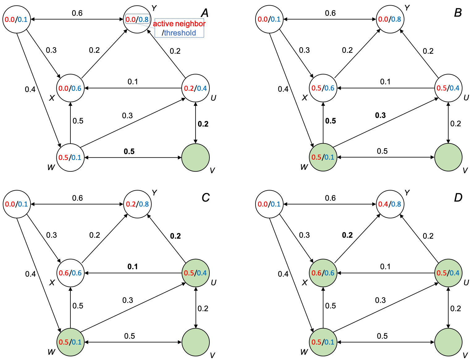
For example, looking at the transition from Panel A to Panel B, we see that an initially active node (off-screen or V) has exerted influence on nodes W and U. In Panel B, W's accumulated influence (0.5) has surpassed its threshold (0.1), so it becomes active. U's influence (0.5) has not yet reached its threshold (0.4) - wait, it has. The diagram shows U's threshold as 0.4 and accumulated influence as 0.5 in panel B. So U should be active. There seems to be an inconsistency in this specific diagram's step-by-step progression, but the principle it illustrates is key: activation occurs when cumulative influence from active neighbors crosses an individual's threshold.
The Independent Cascade Model: A Probabilistic Ripple
The second major model, the Independent Cascade (IC) model, frames influence not as an accumulation of pressure but as a series of probabilistic events. The analogy here is less about social proof and more like the spread of a contagious disease or a piece of gossip.
Formalizing the Independent Cascade (IC) Model
The mechanics of the IC model are quite different from the LT model:
- Each directed edge
(u, v)is assigned a propagation probability, , representing the chance thatuwill successfully transmit the behavior tov. - The process starts with an initial set of "active" nodes.
- In each subsequent step, every node
uthat just became active in the previous step gets a single chance to activate each of its inactive neighborsv. This attempt succeeds with probability . - If the attempt is successful,
vbecomes active in the next step. Whether the attempt succeeds or fails,ucannot try to activatevagain. - The process continues until no new activations occur in a step.
The video lecture we saw earlier also provides a concise definition of this model.
Network Analysis. Lecture 15. Diffusion of innovation and influence maximization.
This segment explains the mechanics of the Independent Cascade model, highlighting its probabilistic nature.
Please watch the explanation of the Independent Cascade model. Pay close attention to the fundamental rule that each node has only one chance to influence its neighbors. This is a critical distinction from both the LT model and standard epidemiological models (like SIS/SIR) where exposure can be continuous.
Comparing the Models and Their Application to Vees
The LT and IC models capture different intuitions about influence.
-
Linear Threshold is well-suited for modeling the adoption of costly or risky behaviors that require significant social proof. In a vee, this could represent a decision to adopt a major new relationship rule (e.g., a new communication protocol, a change in living arrangements). A partner might only agree if they feel both the hinge and their metamour (the other partner) are strongly committed, with the combined influence overcoming their personal threshold of hesitation. The activation rule, which sums influence from all active neighbors, naturally models this need for reinforcement from multiple sources.
-
Independent Cascade is more appropriate for the spread of simple, low-cost information where each exposure provides an independent chance of adoption. This could model the spread of a piece of news or gossip within a polyamorous network. If the hinge tells P1 a story, there's a certain probability P1 believes it and passes it on. The "one chance" rule captures the idea that hearing the same story again from the hinge doesn't necessarily increase the chance of believing it further; the initial attempt is what matters most.
This table provides a quick summary of the key differences:
| Feature | Linear Threshold (LT) Model | Independent Cascade (IC) Model |
|---|---|---|
| Core Mechanism | Accumulation of influence from active neighbors | Probabilistic transmission from newly active nodes |
| Node Parameter | Threshold () | (None) |
| Edge Parameter | Influence weight () | Propagation probability () |
| Activation Condition | A random draw succeeds with probability | |
| Influence Attempts | Continuous influence from all active neighbors at each step | A single attempt from each newly active neighbor |
| Best Analogy | Social reinforcement, peer pressure | Viral contagion, word-of-mouth information spread |
Interestingly, despite their conceptual differences, research has shown that these two models are, in a more general sense, equivalent. This means that for any process described by one model, an equivalent process can be constructed using the other. While the technical details are beyond our scope, it's a powerful result that unifies these two perspectives on diffusion.
Conclusion
In this lesson, we have moved from static network analysis to the dynamics of influence propagation. We described the two foundational models used to understand how behaviors and ideas spread through a social structure.
- Key Takeaways:
- Influence propagation models simulate how a behavior spreads from node to node in a network.
- The Linear Threshold (LT) model assumes activation occurs when the cumulative influence from active neighbors surpasses a node's personal threshold. It models behaviors requiring social reinforcement.
- The Independent Cascade (IC) model assumes activation is a probabilistic event where newly active nodes get one chance to "infect" their neighbors. It models the spread of simple information or low-cost behaviors.
- The choice of model depends on the nature of the "innovation" being spread: LT is for high-threshold, reinforcement-dependent behaviors, while IC is for low-cost, contagious information.
Preview of the next lesson:
Now that we have the theoretical tools, it's time to put them into practice. In our next lesson, we will apply a threshold model to simulate influence propagation in a hypothetical vee network scenario. This will allow us to see how changes in influence weights and individual thresholds can dramatically alter the dynamics of agreement and change within the relationship structure.