Data Types: Continuous vs. Attribute

1. The Two Fundamental Types of Data

In Six Sigma, data is broadly categorized into two families: Continuous and Attribute. Getting this classification right is the first decision you'll make in any data analysis scenario.

Let's begin with some formal definitions and examples.

To summarize and build on that reading:

Continuous Data (also called Variable Data)

This is data that is measured on a scale or continuum. It can be divided into infinitely smaller and more precise units (within the limits of your measurement tool).

Think about key metrics in a manufacturing environment:

• Length: The diameter of a machined shaft in millimeters.
• Time: The cycle time to assemble a component in seconds.
• Temperature: The curing oven temperature in degrees Celsius.
• Pressure: The force applied by a stamping press in kilonewtons (kN).

Continuous data is powerful because it tells you not just if there's a deviation, but also by how much.

Attribute Data (also called Discrete Data)

This is data that is counted or categorized. It places items into distinct buckets.

Attribute data can be further broken down:

• Binary: Only two possible outcomes. Ex: Pass/Fail, Go/No-Go, Yes/No.
• Counts: A count of occurrences. Ex: Number of defects on a car door, number of non-conformances in a batch, number of workplace accidents this month.

Examples in manufacturing include:

• The number of paint scratches on a finished product.
• The result of a visual inspection (e.g., good or bad).
• The number of defective units in a production run.

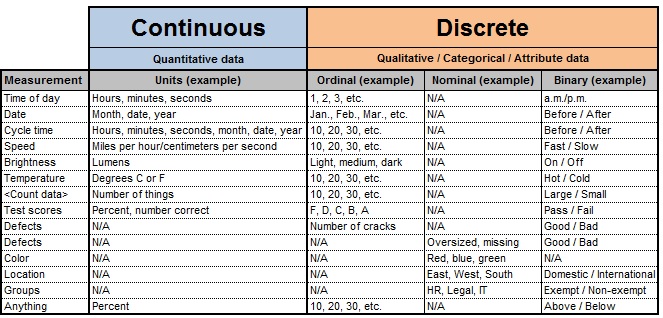
This table provides a helpful visual summary and introduces sub-categories like Ordinal and Nominal, which are useful to know.

2. Why This Distinction Is Crucial

Understanding the difference between continuous and attribute data isn't just an academic exercise. It has profound practical implications for your problem-solving efficiency and your choice of analytical tools.

Information Richness: Getting to the Root Cause Faster

One data type is vastly more powerful for analysis than the other. Let's watch a video that explains why Six Sigma practitioners have a strong preference for continuous data whenever possible.

The key takeaway from the video is powerful:

• Attribute data tells you that you have a problem. (e.g., "We have a 10% defect rate.")
• Continuous data helps you understand the nature of the problem. (e.g., "Is our process centered correctly? Or is our process variation too wide?")

As the video shows, a centering issue can often be fixed quickly, while a variation issue may require a more in-depth project. Attribute data alone cannot tell you which problem you have. This is why continuous data is considered "information-rich."

Guiding Statistical Tool Selection

The second critical reason for classifying data is that it dictates your choice of statistical tools. Using a tool designed for continuous data with attribute data (or vice-versa) will lead to incorrect conclusions.

This is especially evident when selecting Statistical Process Control (SPC) charts, which we will cover in depth later in the course.

This decision process can be visualized with a simple flowchart. At the very top is the first question you must always ask: "Is my data continuous or attribute?"

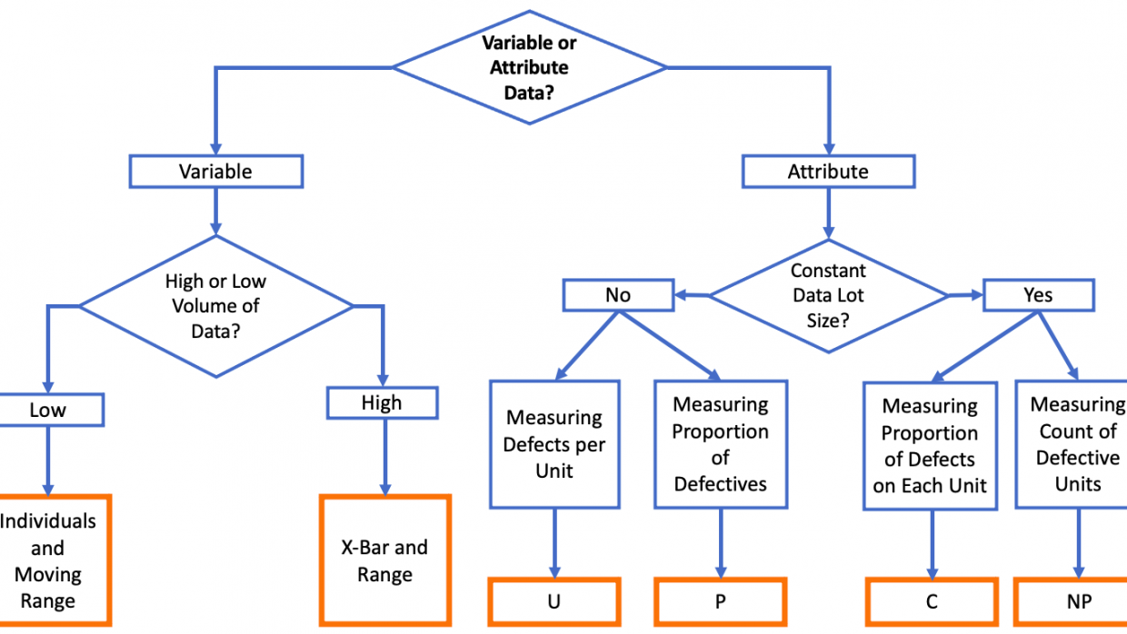
For example, if you are measuring the weight of a product (continuous data), you would follow the path for variable data. If you are counting the number of defective products (attribute data), you would follow a completely different path.

3. Let's Practice: Classifying Manufacturing Data

Now it's your turn. Let's apply these concepts to our brake pad manufacturing scenario. For each of the following metrics, classify it as either Continuous or Attribute.

Scenario Metrics:

1. The hardness of the friction material, measured on the Rockwell scale.
2. The result of a go/no-go gauge test for the brake pad's overall thickness.
3. The weight of a raw material powder in a batch, measured in kilograms.
4. The number of cosmetic blemishes found on a painted caliper.
5. The shift that produced the brake pad (Shift 1, Shift 2, or Shift 3).
6. The time it takes for the curing oven to reach its target temperature, in minutes.
7. A quality auditor's rating of surface finish (Excellent, Good, Poor).
8. The final torque applied to a bolt, measured in Newton-meters (Nm).

Take a few minutes to decide on your answers before revealing the key below.

Finally, it's worth noting that you can convert data from one type to another, but this is usually a one-way street without losing information. You can easily convert continuous data to attribute data (e.g., a diameter of 50.12 mm becomes a "Pass"), but you lose the richness of knowing how good the pass was. Going the other way—from attribute to continuous—isn't about conversion, but about changing what you measure. Instead of noting "Pass/Fail," you would measure the actual dimension.

Conclusion

In this lesson, you've learned the fundamental skill of data classification, which is the gateway to the Measure phase.

Key Takeaways:

• Data is classified into two main types: Continuous (Variable), which is measured, and Attribute (Discrete), which is counted or categorized.
• Continuous data is preferred for root cause analysis because it is "information-rich" and reveals the magnitude and nature of a problem, not just its existence.
• The type of data you have is the primary factor in selecting the appropriate statistical tools, from graphical analysis to control charts and hypothesis tests.

Preview of the Next Lesson:
Now that we understand the types of data we might want to collect, our next step is to plan for it. In the next lesson, you will learn how to create a data collection plan. This plan acts as a recipe, ensuring that the data you gather is accurate, consistent, and useful for your project goals.