Visualizing Process Shifts and Trends with Graphical Tools

1. Comparing Groups with Box Plots

One of the most common tasks in root cause analysis is comparing a continuous output (like part diameter, cycle time, or coating thickness) across different groups or categories (like machines, operators, or shifts). A box plot is the ideal tool for this.

A box plot, or box-and-whisker plot, provides a concise visual summary of a data set's distribution. It displays the median, quartiles, and potential outliers all in one view.

To understand the anatomy of a box plot and how it's used, let's turn to a chapter from a foundational Six Sigma text.

Interpreting Box Plots

As the reading explained, box plots allow for quick, powerful comparisons. When you place two or more box plots side-by-side, you can immediately assess:

• Differences in Location (Central Tendency): Compare the median lines (the line inside the box). A significant difference in the height of the median lines between groups suggests a shift in the process average. For example, if comparing the diameter of parts from two different molds, a difference in medians might indicate one mold is producing consistently larger parts.
• Differences in Variation (Spread): Compare the height of the boxes (the Interquartile Range, or IQR). A taller box indicates more variability within that group. If Shift A's box plot is much taller than Shift B's, it means Shift A's process is less consistent, even if their medians are the same.
• Presence of Outliers: The asterisks highlight individual data points that are statistically unusual. These are often clues to special causes of variation. For instance, an outlier in a cycle time plot could correspond to a specific machine jam or non-standard event that needs investigation.

Imagine you are investigating high defect rates in a soldering process. Your C&E Matrix prioritized two KPIVs: "Soldering Machine" and "Operator". You could create two sets of box plots:

1. A plot of 'Solder Joint Strength' for Machine A vs. Machine B.
2. A plot of 'Solder Joint Strength' for Operator 1 vs. Operator 2 vs. Operator 3.

These plots would instantly show if one machine produces weaker joints on average or if one operator's performance is far more erratic than the others.

2. Dissecting Variation with Multi-Vari Charts

While box plots are excellent for comparing one factor at a time, many manufacturing problems involve the interaction of several factors. This is where the Multi-Vari Chart excels. It is a powerful graphical tool that helps you visualize multiple sources of variation simultaneously.

To use this tool effectively, it's important to understand the different families of variation it's designed to expose.

To summarize the key concepts:

• Positional Variation (Within-Unit): Variation that occurs within a single part or unit. (e.g., thickness at the top vs. the bottom of a molded part).
• Cyclical Variation (Unit-to-Unit): Variation between consecutive units produced. (e.g., the 1st, 2nd, and 3rd parts off a machine in a short time frame).
• Temporal Variation (Time-to-Time): Variation that occurs over longer periods of time. (e.g., differences between Morning Shift, Afternoon Shift, and Night Shift).

A Multi-Vari chart displays all these at once, allowing you to see which "family" of variation is the largest contributor to your problem. Now let's see how to build and read one.

Interpreting a Multi-Vari Chart

Let's look at another example. Imagine you are studying a 'Measurement' from a process with three different 'Operators' who each measure 10 'Units'.

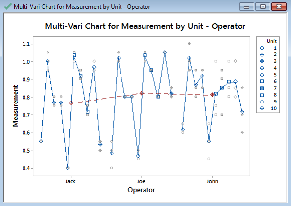
To interpret this chart, you would look for the largest source of variation:

1. Within-Unit Variation: If there were multiple measurements on a single unit, this would be the vertical spread of points for that one unit. (Not shown in this specific chart, but a key concept).
2. Unit-to-Unit Variation (Cyclical): Look at the variation within one operator's group. For "Jack," how much do the averages of the 10 units he measured vary? This represents the inconsistency from one part to the next.
3. Operator-to-Operator Variation (Temporal/Positional): Compare the overall average of each operator. The red dashed line connects these averages. It is clear that the average measurement for "John" is significantly lower than for "Jack" and "Joe".

In this example, the largest source of variation is between operators. This visual evidence strongly suggests that the next step should be to investigate why John's measurements are different. Is it his technique? Is his equipment calibrated differently? The chart doesn't give the answer, but it tells you exactly where to look.

3. Practical Application Exercise

Let's apply these concepts to a scenario. You are investigating inconsistencies in the hardness of a heat-treated gear. Your C&E Matrix has pointed to two KPIVs: Furnace (there are three furnaces in the plant) and Operator (two operators are responsible for loading and running the heat-treat cycle).

You design a small study:

• Response (Y): Hardness (measured in Rockwell C)
• Factor 1 (X1): Furnace (Furnace 1, Furnace 2, Furnace 3)
• Factor 2 (X2): Operator (Alice, Bob)

For each combination (e.g., Alice using Furnace 1), you measure the hardness of 3 consecutive gears.

Your Task (Thought Experiment):

1. Initial Look: What graphical tool would you use to get a quick comparison of the overall performance of the three furnaces, ignoring the operator for a moment? What would you look for?

2. Deeper Dive: What tool would you use to see the influence of the Furnace, the Operator, and the gear-to-gear (cyclical) variation all in one picture?

3. Interpreting the Findings: On your Multi-Vari chart, you see the following:

   • For Furnace 1 and 2, the average hardness is consistently high, regardless of the operator.
   • For Furnace 3, the average hardness is much lower.
   • Within each furnace's results, the points for Alice and Bob are closely clustered together.
   • The variation between the three consecutive gears is minimal in all cases.

   Based on this visual evidence, what is the most likely root cause of the hardness inconsistency?

Conclusion

In this lesson, we explored how to use graphical tools to perform preliminary data analysis. This step is essential for building intuition about your process and forming hypotheses before you conduct formal statistical tests.

Key Takeaways:

• Visual data exploration is a critical bridge between prioritizing potential causes and confirming them with hypothesis testing.
• Box Plots are ideal for comparing the center (median) and spread (IQR) of a continuous variable across different categories of a single factor.
• Multi-Vari Charts provide a more comprehensive view, allowing you to simultaneously visualize and compare multiple sources of variation (positional, cyclical, and temporal) to identify the dominant cause.

Preview of the Next Lesson:

The charts have given us strong visual clues about our root causes. We might see that Machine A produces parts with a lower average diameter than Machine B, or that variation is highest during the night shift. But is that difference "real" or could it just be due to random chance in our sample? In our next lesson, we will address this by learning to select the appropriate hypothesis test based on data type and the objective of the comparison. We will move from visual evidence to statistical proof.