Predictive Modeling: Identifying Process Drivers and Predicting Outcomes

Introduction

In our last lesson, we focused on the critical task of validating a regression model. You learned how to use residual analysis to check the four key assumptions—Linearity, Independence, Normality, and Equal Variance (L.I.N.E.)—ensuring that our model is statistically sound and trustworthy.

Now that we have a validated model, we can confidently put it to use. This lesson is about reaping the benefits of that hard work. We will focus on today's learning outcome: to use a validated regression model to identify vital process drivers and predict outcomes for a given set of parameters.

This is a pivotal step in any Six Sigma project, where we transition from analyzing data to making informed decisions that will improve a process. We'll explore how to interpret the model's output to pinpoint which process inputs have a real impact on our output and then use the model's equation to predict performance and find optimal settings.

Part 1: Identifying the Vital Process Drivers

In any manufacturing process, numerous factors could potentially influence a quality outcome. The goal of regression analysis in the Analyze phase of DMAIC is to sift through these potential causes (the many X's) and identify the "vital few" that truly drive the result (the Y).

A validated regression model provides two key pieces of information for each input variable: its statistical significance (p-value) and the magnitude and direction of its effect (the coefficient).

P-value: As in hypothesis testing, the p-value for a coefficient tells us the probability that the observed effect is due to random chance. A low p-value (typically < 0.05) indicates that the variable is a statistically significant driver of the outcome.
Coefficient: This number quantifies the relationship. A coefficient of +2.5 for Temperature means that for every one-degree increase in temperature, the output Y is predicted to increase by 2.5 units, assuming all other factors are held constant.

Let's begin by reading a short article that outlines the benefits of this process and provides a practical example of how a model is refined to focus only on significant variables.

Step-by-Step Guide to Understanding and Using Multiple Regression

This article from iSixSigma, a respected resource in the field, highlights the key benefits of multiple regression and walks through a clear industry example of identifying significant variables.

Please read two sections from the article: "3 benefits of multiple regression": This section will frame our discussion by summarizing why this analysis is so powerful. "An industry example of multiple regression": Focus on how the team starts with several variables, identifies insignificant ones (like 'number of displays' with its high p-value), and refines the model to focus on the vital drivers ('advertising' and 'trade spend').

As you saw in the example, identifying vital drivers is an iterative process. You might start with a list of potential factors, but your final, most useful model will only contain the ones that are proven to be significant.

Let's look at a typical output from a regression analysis to see where you find this information.

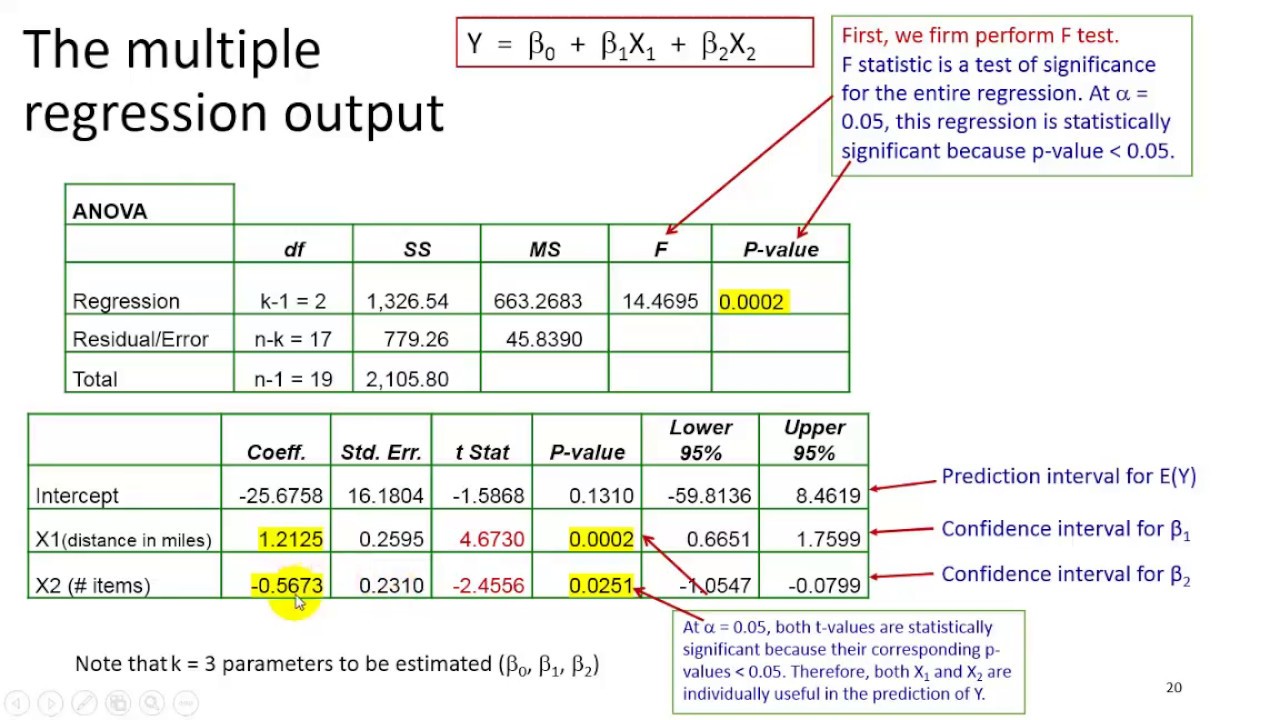
Multiple Regression Output Analysis — This table shows the output from a regression analysis. To identify vital drivers, you would focus on the **P-value** column for each independent variable (X1 and X2). Both have p-values well below 0.05, confirming they are statistically significant drivers of Y.

Once a variable is confirmed as significant, its coefficient tells us the nature of its impact. Understanding this is crucial for process improvement.

Multiple Regression - Interpretation (3of3)

This short video provides a very clear explanation of how to interpret the significance and the practical meaning of the coefficients from a regression output.

Please watch the segment from 08:23 to 11:24. The presenter does an excellent job of explaining how to interpret the coefficient for 'distance' (a positive impact) and 'number of items' (a negative impact), emphasizing the concept of holding other variables constant. This is the essence of understanding process drivers.

Part 2: Predicting Outcomes and Optimizing the Process

Identifying the vital drivers tells us which knobs to turn. The next logical step is to use the model to predict what will happen when we turn them. This is where the regression equation becomes our primary tool for prediction and optimization.

The general form of a multiple regression equation is:

$Y^= b_{0} + b_{1} X_{1} + b_{2} X_{2} + ... + b_{k} X_{k}$

Where:

$Y^$ is the predicted value of the output.
$b_{0}$ is the intercept (the predicted value of Y when all X's are zero).
$b_{1}, b_{2}, ..., b_{k}$ are the coefficients for each independent variable.
$X_{1}, X_{2}, ..., X_{k}$ are the values of the independent variables.

A. Predicting a Specific Outcome

By plugging in a given set of process parameters (X's) into this equation, you can calculate the expected outcome (Y). This is incredibly useful for "what-if" analysis before making physical changes to a process.

Let's review a brief guide that explains how the coefficients are used to form this predictive equation.

Guide: Multiple Regression Analysis

This guide from Learn Lean Sigma clearly explains how the coefficients and intercept from the regression output are used for prediction and decision-making.

Please read the section titled 'Coefficients and Intercept' under 'Interpretation of Results'. Pay close attention to the formula provided for the 'Dependent Variable'. Then, quickly read the final Q&A point, 'How do I interpret the coefficients...?', which gives a great, concise manufacturing example.

B. Optimizing for a Target

Beyond predicting the result for one set of inputs, we can use the model to find the optimal combination of inputs to achieve a specific target. For example, what settings for speed and feed rate will minimize surface roughness?

Statistical software like Minitab has built-in tools that make this easy. They use the regression model to search for the input settings that best achieve your goal, whether it's minimizing, maximizing, or hitting a specific target value.

The following video demonstrates this entire process using Minitab's Assistant, which is designed to guide you through the analysis.

How to Conduct a Multiple Regression study using Minitab 17

This video from RMK Six Sigma is a perfect practical demonstration of our learning outcome. It shows how to use Minitab to build a model, identify significant factors, and, most importantly, use the optimization tool to find the right settings for a target outcome.

Please watch the following segments: Model Equation (08:47 - 10:11): Observe how the software presents the final regression equation derived from the data. This is the mathematical model we'll use for prediction. Prediction and Optimization (10:11 - 11:32): This is the key part. Notice how the user has specified a target response of 200, and Minitab's 'Prediction and Optimization Report' provides the exact settings for the significant predictors to achieve this target, along with a prediction interval.

Tying It All Together: A Manufacturing Scenario

Let's solidify these concepts with a practical example.

Imagine you're working to improve the seal strength of a plastic package. After running a regression analysis, your validated model is:

Seal Strength (N) = 10.5 - 0.25 * Line_Speed + 0.80 * Temperature + 0.12 * Pressure

The p-values from your output were:

Line_Speed: 0.03 (Significant)
Temperature: 0.001 (Significant)
Pressure: 0.45 (Not Significant)

Let's answer a few questions:

Identify the Vital Drivers: Which factors are the vital drivers of seal strength?
- Answer: Line_Speed and Temperature are the vital drivers because their p-values are less than 0.05. Pressure is not a significant factor.
Interpret the Drivers: To increase seal strength, how should you adjust the line speed and temperature?
- Answer: You should decrease Line_Speed (due to the negative coefficient of -0.25) and increase Temperature (due to the positive coefficient of +0.80).
Predict an Outcome: Your current process settings are a Line_Speed of 10 m/min and a Temperature of 150°C. What is the predicted seal strength?
- Answer:
  $Seal Strength = 10.5 - (0.25 \times 10) + (0.80 \times 150)$
  $Seal Strength = 10.5 - 2.5 + 120$
  $Seal Strength = 128 N$

This simple exercise demonstrates the power of a regression model: it guides you on where to focus your efforts and allows you to predict the results of your changes.

Conclusion

In this lesson, we completed our journey with regression analysis by learning how to apply a validated model to achieve practical results. This is the ultimate goal of building a model in a Lean Six Sigma project.

Key Takeaways:

Vital Process Drivers are the input variables (X's) with a statistically significant impact on the output (Y), identified by p-values < 0.05 in the regression output.
Coefficients in the regression equation quantify the relationship, telling you the magnitude and direction of change in Y for a one-unit change in X.
The Regression Equation is a powerful tool for prediction, allowing you to perform "what-if" analyses and forecast process outcomes based on specific input settings.
Optimization tools in statistical software use the regression model to find the ideal settings for your vital drivers to achieve a desired target, such as maximizing yield or minimizing defects.

Preview of the Next Lesson:

Regression analysis is excellent for modeling relationships in an existing process using historical or observational data. However, sometimes we need to proactively test factors and their interactions in a structured way. This leads us to our next major topic: Design of Experiments (DOE). In the next lesson, we will introduce the fundamental principles of DOE, including factors, levels, responses, and randomization, which will allow you to efficiently and effectively experiment to find optimal process conditions.

Recommended resources