Hello. In the previous lesson, you used boundary invariants to make binary search correct on every edge case. That gave you an asymptotic answer——to the question “how does this algorithm scale?” Profiling answers a different, practical question: where did this particular run actually spend its time?
This final lesson in the first DSA module introduces a workflow you can reuse for Python data-processing and evaluation code: profile a representative function, interpret cProfile and pstats output, identify the dominant bottleneck rather than its innocent-looking caller, make one targeted change, and measure again. Plan for about 40 minutes.
Profile before optimizing
It is easy to guess incorrectly about performance. A preprocessing function may contain Python loops, string handling, sorting, file reads, and calls into libraries. Improving the most visibly “inefficient” line might make no observable difference if it accounts for only 2% of runtime.
A profiler replaces guesses with measurements. Python’s standard cProfile profiler records function calls and timing statistics during an execution. It is especially useful for the kind of orchestration code common in an ML pipeline: manifest construction, feature preparation, evaluation aggregation, or repeated Python-side transforms.
The Python Profilers — Python 3.14.2 documentation
Read the relevant parts of the official Python documentation to establish what cProfile measures and how its reports should be read. The documentation is the primary reference here; focus on the distinction between profiling and benchmarking, then on the timing columns and sort modes.
In “Introduction to the profilers,” read the opening explanation of deterministic profiling. Pay particular attention to the purpose distinction: use a profiler to locate time-consuming program structure, rather than to make precise microbenchmark claims. Next, in “Instant User’s Manual,” begin at the paragraph starting “To profile a function that takes a single argument” and read through the explanation of the report columns. Study the column definitions, especially tottime and cumtime. Finally, continue in the subsection explaining pstats.Stats. Find the examples using SortKey.CUMULATIVE and SortKey.TIME; read the sorting guidance. Notice that the two sort orders answer different diagnostic questions.
A key boundary to keep in mind:
- Profiling asks: Which parts of this representative workload consume runtime?
- Benchmarking asks: How fast is a small operation, accurately and repeatably?
cProfile adds measurement overhead, so do not use it to decide whether one expression is 3% faster than another. Use it to find the large regions of work that deserve attention. After a targeted fix, use ordinary end-to-end timing as a sanity check that the whole workload improved.
A concrete workload: repeated scans in an audio manifest summary
Consider a simplified manifest operation. Suppose each row represents an audio example and contains a speaker identifier and a sample count. We want the number of examples for each speaker and the total number of samples.
The following implementation is correct, but it hides a repeated full-dataset scan:
def count_examples_for_speaker(rows: list[dict], speaker: str) -> int:
    count = 0

    for row in rows:
        if row["speaker"] == speaker:
            count += 1

    return count


def speaker_counts_naive(rows: list[dict]) -> dict[str, int]:
    speakers = {row["speaker"] for row in rows}

    return {
        speaker: count_examples_for_speaker(rows, speaker)
        for speaker in speakers
    }


def build_manifest_summary(rows: list[dict]) -> dict:
    counts = speaker_counts_naive(rows)
    total_samples = sum(row["num_samples"] for row in rows)

    return {
        "num_examples": len(rows),
        "num_speakers": len(counts),
        "speaker_counts": counts,
        "total_samples": total_samples,
    }
If there are rows and distinct speakers, then count_examples_for_speaker() scans rows once for every speaker. The dominant part is therefore approximately:
This may be harmless for a few speakers, but costly for a large corpus with many speakers. Crucially, you should not conclude that it is the bottleneck merely by reading the code. First, profile it under a workload that resembles the data volume and distribution you care about.
Create synthetic rows outside the profiled function so that your report measures the summary operation, not data creation:
def make_rows(
    num_rows: int = 50_000,
    num_speakers: int = 100,
) -> list[dict]:
    return [
        {
            "speaker": f"speaker_{index % num_speakers}",
            "num_samples": 16_000 * (1 + index % 8),
        }
        for index in range(num_rows)
    ]


rows = make_rows()
Now use the object-oriented cProfile API:
import cProfile
import pstats
from pstats import SortKey

profiler = cProfile.Profile()

summary = profiler.runcall(build_manifest_summary, rows)

profiler.dump_stats("manifest_summary.prof")

stats = pstats.Stats(profiler)
stats.strip_dirs().sort_stats(SortKey.CUMULATIVE).print_stats(15)
runcall() profiles only the supplied function call. This makes the profiling scope explicit: you are measuring build_manifest_summary(rows), not interpreter startup, synthetic-data generation, or unrelated setup code.
The saved manifest_summary.prof file is useful when you want to revisit the report later:
import pstats
from pstats import SortKey

(
    pstats.Stats("manifest_summary.prof")
    .strip_dirs()
    .sort_stats(SortKey.CUMULATIVE)
    .print_stats(15)
)
You can also profile a complete script from the command line:
python -m cProfile -o manifest_summary.prof manifest_summary.py
For interview-style problems, profiling is usually unnecessary: first reason about the complexity. For a real data or evaluation pipeline, use both. Complexity predicts scaling; profiling tells you what dominates the observed workload now.
How to read the report
A cProfile report has rows resembling this. The precise times will differ by machine, Python version, and workload, so treat the numbers as illustrative.
         106 function calls in 1.28 seconds

   ncalls  tottime  percall  cumtime  percall  filename:lineno(function)
        1    0.00    0.00    1.28    1.28  manifest.py:22(build_manifest_summary)
        1    0.01    0.01    1.23    1.23  manifest.py:13(speaker_counts_naive)
      100    1.18    0.01    1.18    0.01  manifest.py:1(count_examples_for_speaker)
        1    0.03    0.03    0.03    0.03  {built-in method builtins.sum}
The important columns are:
| Column | Meaning | Useful diagnostic question |
|---|---|---|
ncalls |
Number of calls | Is this work repeated unexpectedly? |
tottime |
Time spent in the function’s own body, excluding called functions | Is this function itself a hot loop or blocking operation? |
cumtime |
Time in the function plus all functions it calls | Which high-level operation owns most of the runtime? |
percall |
Average time per call | Is each call expensive, or is a cheap call repeated too often? |
The top-level function, build_manifest_summary, has the greatest cumulative time. That is expected: it encloses the whole workload. It is not yet a useful diagnosis. Rewriting the wrapper function without changing the work beneath it will not materially improve performance.
Instead, follow the expensive cumulative-time path downward:
build_manifest_summaryowns almost all runtime.- Its child
speaker_counts_naiveowns almost all runtime. - The leaf function
count_examples_for_speakerhas the largesttottime. - It was called 100 times, and every call scans all rows.
The dominant runtime bottleneck is therefore:
Repeatedly scanning the complete manifest inside
count_examples_for_speaker, once per speaker.
This is more precise than saying “the summary function is slow.” It identifies both the location and the mechanism: a nested scan causing an pattern.
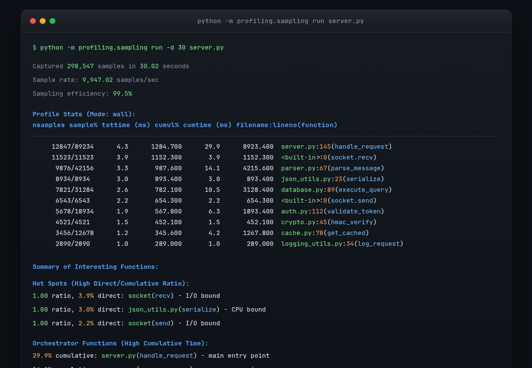
Two sort orders, two complementary views
Start with cumulative time:
stats.sort_stats(SortKey.CUMULATIVE).print_stats(15)
This answers:
Which high-level paths account for the application’s elapsed time?
Then sort by internal, or self, time:
stats.sort_stats(SortKey.TIME).print_stats(15)
This answers:
Which function bodies spend the most time directly in their own code?
In the manifest example, cumulative time reveals that speaker counting dominates the summary path; internal time confirms that the repeated row-scanning function does the work itself.
A third useful pattern is a high call count. A function with small percall time may still be dominant if called hundreds of thousands of times. In an ML pipeline, this often points to Python-level per-item work that could be batched, cached, or replaced with a single pass over data.
How To FIND SLOW CODE In Python & OPTIMIZE IT (FT. cProfile)
Watch this short demonstration from Indently to see a profile report interpreted in practice. It reinforces the distinction between total/self time and cumulative time, then shows why the profiler should guide a targeted optimization rather than a broad rewrite.
Watch the first report to see cProfile run on a main function and sorted by cumulative time. Then watch the time comparison, focusing on the explanation of a function’s own work versus time spent in its callees. Map that distinction onto speaker_counts_naive and count_examples_for_speaker in the manifest example.
Confirm the cause, then make one targeted change
Once profiling has isolated the repeated scan, the repair follows directly from the diagnosis. Count each speaker while traversing the rows once:
def speaker_counts_one_pass(rows: list[dict]) -> dict[str, int]:
    counts: dict[str, int] = {}

    for row in rows:
        speaker = row["speaker"]
        counts[speaker] = counts.get(speaker, 0) + 1

    return counts
Replace this line:
counts = speaker_counts_naive(rows)
with:
counts = speaker_counts_one_pass(rows)
The updated summary operation performs one pass to build speaker counts and one pass for total_samples:
You could combine both aggregations into one loop later, but do not start by making several unrelated changes. The first goal is to validate the hypothesis:
Replacing repeated full-manifest scans with one-pass aggregation substantially reduces runtime while preserving the returned summary.
Before timing anything, verify behavioral equivalence:
assert speaker_counts_naive(rows) == speaker_counts_one_pass(rows)
Then profile the revised build_manifest_summary(rows) with the same rows object and the same profiling scope. A successful new profile should show:
count_examples_for_speakerno longer appears on the dominant path;- the overall cumulative time of
build_manifest_summarydrops; - another operation may now become the largest remaining cost.
That final point matters. Optimization is iterative: removing one bottleneck often exposes the next one. Do not assume a function remains dominant after the workload or implementation changes.
When tottime and cumtime tell different stories
Consider these common cases:
| Profile pattern | Likely interpretation | Next step |
|---|---|---|
High cumtime, low tottime |
A wrapper mostly delegates work | Inspect its expensive callees |
High tottime, high cumtime |
The function’s own body is expensive | Inspect loops, algorithm, allocations, or blocking call |
Very high ncalls, low percall |
Repeated small overhead | Reduce call frequency, batch work, or cache results |
| Built-in I/O call dominates | Waiting on storage, network, or OS activity | Investigate data access pattern, concurrency, caching, or transfer volume |
| A numerical-library call dominates | The expensive work is in a native implementation | Confirm input sizes and algorithm choice before trying to rewrite Python around it |
A deterministic profiler sees Python function-call structure very well. For heavy native kernels or accelerator execution, it may show a Python-level call as one large aggregate rather than explain the kernel-level cause. In that situation, you would need a system- or framework-specific profiler; later in this course, you will apply that distinction to PyTorch workloads. For now, cProfile is exactly the right first tool for ordinary Python control flow and data processing.
A compact profiling protocol
Use this procedure whenever a Python function feels slow:
- Define the workload. Use representative input size, distribution, and code path.
- Scope the profile. Profile the specific operation, excluding irrelevant setup when possible.
- Sort by
cumtime. Find the expensive execution path, not merely the entry point. - Sort by
tottime. Locate expensive function bodies or blocking operations. - Check
ncalls. Look for surprising repetition. - State a causal hypothesis. For example: “This function scans all rows once per speaker.”
- Change one cause. Avoid a large, untestable rewrite.
- Verify correctness and re-profile on the same workload.
This combines the discipline of algorithmic analysis with actual runtime evidence. It is also a strong interview habit: rather than saying “I optimized the code,” you can explain what you measured, what you inferred, and how you validated the improvement.
Key takeaways
cProfile helps identify where a Python execution spends time; it is a diagnostic profiler, not a microbenchmarking tool.
- Use
cProfile.Profile().runcall(...)to profile a precisely chosen function invocation. - Save results with
dump_stats()and inspect them withpstats.Stats. - Sort by
SortKey.CUMULATIVEto find expensive call paths, and bySortKey.TIMEto find functions expensive in their own bodies. - Do not mistake a top-level wrapper with high cumulative time for the true bottleneck. Follow the call path to the costly child or leaf operation.
- Treat
ncallsas evidence: many cheap calls can dominate total runtime. - A valid optimization workflow is: profile, state a hypothesis, make one causal change, verify output, and profile again.
- In the manifest example, repeated full-dataset scans create an bottleneck; one-pass counting reduces that component to .
You have now completed the core Python DSA patterns module. Next, the course shifts to the mathematical foundations needed to implement and reason about ML models, beginning with vector and matrix operations while tracking tensor shapes.