Welcome back. In the previous lesson, stacks worked because you could state exactly what was still unresolved at every step. Binary search needs the same discipline: its idea is simple, but implementations fail when the boundaries do not have a precise meaning.
In this lesson, you will implement binary search as a boundary-finding algorithm. Rather than memorizing a while condition and a few +1 or -1 updates, you will define what low and high guarantee, preserve those guarantees, and obtain a deterministic result even for empty arrays, missing targets, and duplicates.
Plan for about 40 minutes: work through the implementation and traces, watch the short visual explanation, then run the verification cases.
Binary search begins with a contract
Binary search applies only when the sequence is sorted according to the same comparison you use in the search.
For an ascending integer list, such as:
values = [1, 3, 3, 3, 5, 8]
suppose the target is 3. An ordinary “find any matching index” contract is ambiguous because indices 1, 2, and 3 all match.
A more useful and fully defined contract is:
Return the first position where
targetcan be inserted without breaking sorted order.
This position is called the lower bound, and Python exposes the same behavior as bisect_left().
For a list of length , the returned insertion index can be anywhere from through , inclusive:
- : the target belongs before every element.
- an index within the array: the target belongs there, possibly before duplicates.
- : the target belongs after every element.
For values = [1, 3, 3, 3, 5, 8]:
| Target | Lower-bound index | Meaning |
|---|---|---|
0 |
0 |
Insert before 1 |
3 |
1 |
Insert before the first 3 |
4 |
4 |
Insert between 3 and 5 |
9 |
6 |
Insert after 8 |
This contract is stronger than “find it or return -1.” It always produces a meaningful answer, even when the target is absent.
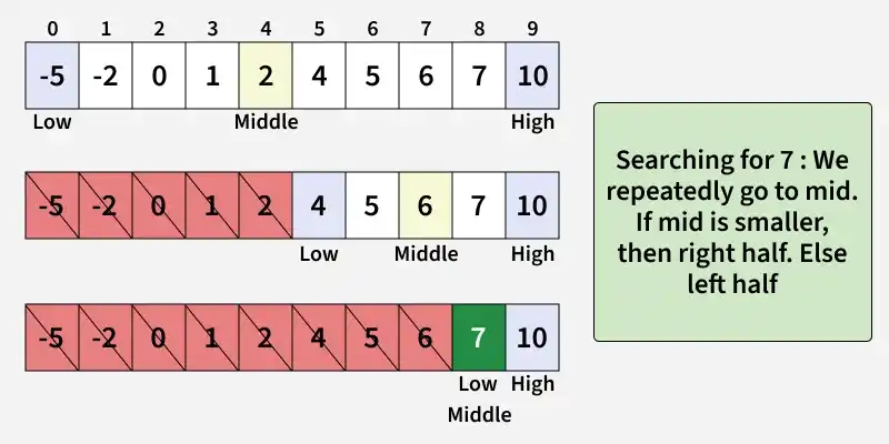
The image captures the central efficiency idea: each comparison eliminates about half of the remaining possibilities. But the important implementation question is: what exactly remains possible after each update?
The invariant: what the boundaries promise
We will use a half-open candidate interval:
That includes low but excludes high.
Initialize it as:
low, high = 0, len(values)
Notice that high is the array length, not the final valid index. This is intentional: index len(values) represents a valid insertion position.
For a target x, the lower-bound invariant is:
- Every index strictly before
lowstores a value smaller thanx. - Every index at or after
highstores a value greater than or equal tox. - Therefore, the lower-bound answer remains somewhere in .
Written more formally:
At initialization:
low = 0
high = len(values)
both claims are true vacuously:
- There are no indices before
0. - There are no array indices at or beyond
len(values).
This is a good sign: an invariant should be true before the loop begins, not merely become true later.
The core implementation
def lower_bound(values: list[int], target: int) -> int:
    """
    Return the first index where target can be inserted
    while preserving ascending sorted order.
    """
    low, high = 0, len(values)

    # Invariant:
    # - values[i] < target for every i < low
    # - values[i] >= target for every i >= high
    while low < high:
        mid = low + (high - low) // 2

        if values[mid] < target:
            low = mid + 1
        else:
            high = mid

    return low
There are only two branches because every middle element is either:
- too small:
values[mid] < target, or - large enough:
values[mid] >= target.
The update logic follows directly from the invariant.
If the middle value is too small
if values[mid] < target:
    low = mid + 1
Because the list is sorted, if values[mid] < target, then every index up to and including mid is too small. The insertion point cannot be mid or anything to its left.
So the next valid lower boundary is:
If the middle value is large enough
else:
    high = mid
If values[mid] >= target, then mid itself might be the first valid insertion position. We must keep it as a candidate.
So we move high to mid, rather than mid - 1.
That missing -1 is one of the most important details in this version of binary search.
Trace the invariant with duplicates
Consider:
values = [1, 3, 3, 3, 5, 8]
target = 3
We expect the answer to be index 1, the first 3.
| Step | low |
high |
mid |
values[mid] |
Decision |
|---|---|---|---|---|---|
| Start | 0 |
6 |
— | — | Entire insertion range is possible |
| 1 | 0 |
6 |
3 |
3 |
Large enough, so high = 3 |
| 2 | 0 |
3 |
1 |
3 |
Large enough, so high = 1 |
| 3 | 0 |
1 |
0 |
1 |
Too small, so low = 1 |
| End | 1 |
1 |
— | — | Return 1 |
When the loop ends, low == high. The two boundary statements combine:
- every index before
1is smaller than3; - every index from
1onward is at least3.
That uniquely identifies index 1 as the lower bound.
Now try a missing target:
values = [1, 3, 3, 3, 5, 8]
target = 4
The algorithm returns 4. It does not claim that 4 exists. It says that index 4 is where 4 belongs:
[1, 3, 3, 3, 4, 5, 8]
            ^
          index 4
This is why lower-bound binary search is a robust primitive: the search result and the insertion result are the same operation.
Binary Search - A Different Perspective | Python Algorithms
Watch “Binary Search - A Different Perspective” by mCoding. It presents the same lower-bound viewpoint: binary search finds a transition from “too small” to “large enough,” rather than merely looking for an equal value.
Start with the insertion viewpoint, which makes missing values, duplicates, and empty arrays unambiguous. Then watch the predicate view to see why sortedness creates a true-to-false boundary. Continue with the implementation, paying close attention to why a true middle value moves the lower bound to mid + 1, while a false middle value keeps mid by moving the upper bound to mid. Watch the termination argument for the reasoning that rules out an infinite loop. Finally, after the brief transition, watch bisect variants to connect the implementation to Python’s standard library.
From insertion position to exact search
Many interview prompts ask for an index if the target exists and -1 otherwise. You can derive that safely from lower_bound().
def find_first_index(values: list[int], target: int) -> int:
    index = lower_bound(values, target)

    if index < len(values) and values[index] == target:
        return index

    return -1
This returns the leftmost occurrence when duplicates exist:
values = [1, 3, 3, 3, 5, 8]

find_first_index(values, 3)  # 1
find_first_index(values, 4)  # -1
find_first_index(values, 8)  # 5
The post-search check is essential:
index < len(values) and values[index] == target
lower_bound() always returns an insertion point, but an insertion point is not necessarily a matching element.
For example:
lower_bound([1, 3, 3, 3, 5, 8], 4) # 4
At index 4, the value is 5, not 4.
The predicate perspective
The comparison:
values[mid] < target
can be viewed as a Boolean predicate:
is_too_small = values[mid] < target
For:
values = [1, 3, 3, 3, 5, 8]
target = 4
the predicate values across the array are:
| Value | 1 |
3 |
3 |
3 |
5 |
8 |
|---|---|---|---|---|---|---|
value < 4 |
True | True | True | True | False | False |
Binary search finds the first False.
This is the deeper requirement behind binary search: not merely “an array is sorted,” but that the condition being tested changes monotonically from one region to another. In this lesson, sorting guarantees that monotonic structure.
Do not apply this search to arbitrary unsorted model scores or arbitrary audio segments just because they are numeric. A sequence such as:
[1, 7, 3, 9]
does not produce a reliable “smaller values, then larger values” boundary for most targets.
Why it terminates and why it is logarithmic
A correct binary-search loop needs both a correctness argument and a progress argument.
Correctness: the answer is never discarded
Let be the true lower-bound index.
- If
values[mid] < target, sortedness proves that . Updatinglow = mid + 1keeps in the candidate interval. - Otherwise,
values[mid] >= target, so . Updatinghigh = midkeeps in the candidate interval.
Thus, every update preserves the invariant.
Progress: the interval strictly shrinks
The loop runs only while:
low < high
Therefore:
mid = low + (high - low) // 2
always satisfies:
- In the too-small branch,
lowbecomesmid + 1, which is strictly larger than the oldlow. - In the large-enough branch,
highbecomesmid, which is strictly smaller than the oldhigh.
So the interval cannot remain unchanged. Eventually, low == high, and the loop stops.
Each iteration roughly halves the active interval. For an array of length , the time complexity is:
The iterative implementation uses only a few index variables, so its auxiliary space complexity is:
A practical caveat: if the input is not already sorted and you sort it solely to perform one search, sorting costs:
Binary search is most valuable when the data is already sorted, or when you will make many searches against the same sorted collection.
Boundary conventions: choose one and do not mix them
There is nothing inherently wrong with the traditional inclusive-range form of binary search. The bugs happen when code combines rules from two different conventions.
| Convention | Initial bounds | Loop condition | Meaning of high |
|---|---|---|---|
| Exact-search interval | left = 0, right = n - 1 |
left <= right |
Last valid array index |
| Lower-bound interval | low = 0, high = n |
low < high |
First excluded candidate insertion position |
In the lower-bound implementation, these choices must stay together:
low, high = 0, len(values)

while low < high:
    mid = low + (high - low) // 2

    if values[mid] < target:
        low = mid + 1
    else:
        high = mid
Common mistakes are easier to diagnose in terms of violated invariants:
-
Using
high = mid - 1in lower-bound search
This discardsmideven though it may be the first valid insertion position. -
Using
low = midwhen the middle is too small
Ifhigh = low + 1, thenmid == low; assigninglow = midmakes no progress and can loop forever. -
Setting
high = len(values)but usingwhile low <= high
Eventually,midmay equallen(values), which is not a valid list index. -
Returning
lowas an exact-match answer without checking the value
The returned position may be an insertion point for a missing target. -
Using the wrong equality policy with duplicates
For the first occurrence, equality belongs in thehigh = midbranch because equal values are “large enough.”
Verify the implementation against edge cases
Run this compact test harness after writing the functions:
test_cases = [
    ([], 4, 0),
    ([1, 3, 3, 3, 5, 8], 0, 0),
    ([1, 3, 3, 3, 5, 8], 3, 1),
    ([1, 3, 3, 3, 5, 8], 4, 4),
    ([1, 3, 3, 3, 5, 8], 9, 6),
]

for values, target, expected in test_cases:
    actual = lower_bound(values, target)
    assert actual == expected, (values, target, actual, expected)

assert find_first_index([], 4) == -1
assert find_first_index([1, 3, 3, 3, 5, 8], 3) == 1
assert find_first_index([1, 3, 3, 3, 5, 8], 4) == -1
In production Python code, prefer the standard-library implementation when manual implementation is not required:
from bisect import bisect_left

values = [1, 3, 3, 3, 5, 8]
index = bisect_left(values, 3)  # 1
To use it as an exact search, retain the same post-check:
index = bisect_left(values, target)

if index < len(values) and values[index] == target:
    print("Found at", index)
else:
    print("Not found")
For an interview, implementing the loop yourself demonstrates that you understand the invariant. In application code, using bisect_left() avoids reintroducing boundary bugs in a well-tested standard operation.
Key takeaways
Binary search becomes reliable when you define the boundary contract before writing the loop.
- A sorted array gives a monotonic split between values that are too small and values that are large enough.
lower_bound()returns the first valid insertion position, including for missing targets, duplicates, and empty arrays.- With the half-open convention, initialize
low = 0andhigh = len(values). - Maintain the invariant that values before
loware too small, while values fromhighonward are large enough. - When
values[mid] < target, setlow = mid + 1; otherwise sethigh = mid. - Convert a lower-bound result into exact search with a bounds check and equality check.
- Binary search runs in time and uses auxiliary space.
Next, you will shift from asymptotic reasoning to measurement: profiling a Python function to locate its dominant runtime bottleneck.