Problems with the Big Bang Model

1. The Flatness Problem: A Universe on a Knife's Edge

Our cosmological measurements, particularly from the CMB, tell us that the universe today is very nearly spatially flat. The density parameter is incredibly close to one:

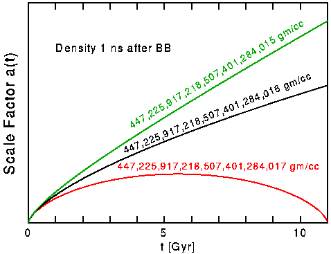
The flatness problem is the puzzle of why this is the case. To understand why it's a puzzle, we need to see how $\Omega$ evolves with time. From the Friedmann equation, we derived the following key relation:

Notice that for a flat universe ($k=0$), $\Omega$ is always exactly 1. However, if there is any deviation from $\Omega =1$, no matter how small, that deviation grows over time.

• During the radiation-dominated era, $a(t)\propto t^{1/2}$, so $H=\dot{a}/a\propto t^{-1}$. This means $a^2{H}^2\propto t^{-1}$, and thus $|\Omega (t)-1|\propto t$.
• During the matter-dominated era, $a(t)\propto t^{2/3}$, so $H\propto t^{-1}$. This means $a^2{H}^2\propto t^{-4/3}{t}^2=t^{-2/3}$, and thus $|\Omega (t)-1|\propto t^{2/3}$.

In both epochs, any initial deviation from $\Omega =1$ grows with time. This means that for $\Omega$ to be close to 1 today, after 13.8 billion years of evolution, it must have been astonishingly close to 1 in the early universe. The state $\Omega =1$ is an unstable equilibrium point, like a pencil balanced perfectly on its tip. Any slight nudge causes it to fall away rapidly.

To fully appreciate the scale of this fine-tuning, let's watch a detailed derivation by Professor Alan Guth, one of the original proponents of the inflationary theory.

As the video demonstrates, for ${\Omega }_0$ to be within a few percent of 1 today, its value at $t=1$ second must have been tuned to 1 with an accuracy of about one part in $10^{18}$:

The standard Big Bang model offers no explanation for this extraordinary initial condition. It must be put in by hand. This is the essence of the flatness problem.

2. The Horizon Problem: A Puzzling Uniformity

The most precise picture we have of the early universe comes from the Cosmic Microwave Background (CMB). The CMB is the thermal radiation from the era of recombination, when the universe was about 370,000 years old. The most striking feature of the CMB is its near-perfect isotropy: it has the same temperature ($T\approx 2.725$ K) in all directions, with tiny fluctuations of only one part in $10^5$.

This uniformity suggests that the plasma at the time of recombination was in thermal equilibrium. However, in the standard Big Bang model, this presents a major causal dilemma. When we look at two opposite points in the sky, we are seeing regions of the early universe that, according to the model, were too far apart to have ever exchanged light or any other causal signal. How, then, did they "know" to have the same temperature?

Let's walk through the calculation. The question is: what was the maximum distance a light signal could have traveled from the Big Bang ($t=0$) until the time of decoupling ($t_d$)? This is the particle horizon, $d_H(t_d)$. For a matter-dominated universe (a good approximation for that epoch), this is $d_H(t_d)\approx 3c{t}_d$.

Now, we compare this to the actual physical distance, at time $t_d$, between two points on the CMB that are on opposite sides of our sky.

As Guth shows, the calculation reveals that two points on opposite sides of our sky were separated by about 46 horizon distances at the time the CMB was emitted. There was no time for any physical process, limited by the speed of light, to smooth out temperature differences between them.

The standard Big Bang model cannot explain this large-scale uniformity; it must simply be assumed as an initial condition. This is the horizon problem.

3. The Magnetic Monopole Problem: Unseen Relics

The third problem is of a different character, as it arises from combining cosmology with ideas from high-energy particle physics, specifically Grand Unified Theories (GUTs). Your interests in particle physics and gauge theories will be relevant here.

GUTs propose that at extremely high energies ($\sim 10^{16}$ GeV), the strong, weak, and electromagnetic forces unify into a single force described by a larger gauge group (e.g., SU(5)). As the universe expanded and cooled below the GUT energy scale, this symmetry was spontaneously broken.

A generic prediction of this symmetry-breaking process is the formation of topological defects—stable, particle-like objects. In the case of GUTs, these defects are predicted to be magnetic monopoles: particles with a net magnetic charge (an isolated north or south pole).

Here's the problem:

1. Massive: GUT monopoles are predicted to be incredibly heavy, with a mass $m_M\sim 10^{16}$ GeV/c${}^2$.
2. Abundant: The standard model predicts that roughly one monopole should be formed per horizon volume at the time of the GUT phase transition.
3. Stable: They are thought to be stable and would survive to the present day.

When you calculate the expected number density of these monopoles today, their contribution to the total energy density of the universe would be many orders of magnitude larger than the critical density (${\Omega }_M\gg 1$). This would have caused the universe to recollapse long ago. Yet, despite extensive searches, not a single magnetic monopole has ever been definitively observed. This glaring contradiction between the prediction of GUTs and cosmological observation is the magnetic monopole problem.

Conclusion

Today we have explored three profound puzzles that arise within the standard Hot Big Bang model. It is crucial to understand that these are not proofs that the model is "wrong," but rather strong indications that it is incomplete.

Key Takeaways:

• The Flatness Problem: The universe today is observed to be nearly flat ($\Omega \approx 1$). Since $\Omega =1$ is an unstable equilibrium point, this requires the initial density of the universe to have been fine-tuned to the critical density with incredible precision.
• The Horizon Problem: The CMB is observed to be at a uniform temperature across the entire sky, yet in the standard model, regions separated by more than $\sim 1^{\circ }$ were causally disconnected at the time the CMB was formed. There was no time for thermal equilibrium to be established.
• The Monopole Problem: Grand Unified Theories, a leading candidate for physics beyond the Standard Model, predict the copious production of massive, stable magnetic monopoles in the early universe. Their predicted density today would vastly over-close the universe, in stark contradiction to observations.

These three seemingly disconnected problems—one of geometry, one of causality, and one of particle relics—all point to a missing piece in our understanding of the universe's first fraction of a second. As we will see, a single, elegant idea has the potential to solve all three at once.

Preview of Next Lesson:

In our next lesson, we will formally introduce Cosmic Inflation. We will see how a brief, dramatic period of super-accelerated expansion in the first moments after the Big Bang can naturally drive the universe to flatness, stretch a single tiny causal patch to encompass our entire observable universe, and dilute the density of any unwanted relics to near zero, thus resolving all three problems we discussed today. We will introduce the simplest model for this process, a scalar field called the "inflaton," and derive its equations of motion.