Extrinsic Curvature of a Spatial Slice

1. Intrinsic vs. Extrinsic Curvature: A Geometric Picture

Before diving into the formalism, it's essential to build an intuition for what "extrinsic curvature" means, and how it differs from the intrinsic curvature (the Riemann tensor of the slice, ${}^{(3)}{R}_{\alpha \beta \gamma \delta }$) which you've studied before.

• Intrinsic curvature can be measured by an "ant" living entirely within a surface, without any knowledge of a higher dimension. For example, by walking in a triangle and measuring the sum of the angles, the ant can determine if its surface is curved.
• Extrinsic curvature measures how a surface is bent or embedded within a higher-dimensional space. An observer in the higher-dimensional space can see this bending.

As the examples show:

• A plane is flat both intrinsically ($R=0$) and extrinsically ($K=0$).
• A cylinder is intrinsically flat ($R=0$)—you can unroll it into a flat plane without tearing it. However, it is extrinsically curved ($K\ne 0$) within 3D space.
• A sphere is curved both intrinsically ($R\ne 0$) and extrinsically ($K\ne 0$).

The extrinsic curvature $K_{ij}$ of our spatial slice ${\Sigma }_t$ captures precisely this bending of the 3D space within the 4D spacetime. Geometrically, it measures how the future-pointing unit normal vector field $n^{\mu }$ changes as we move from one point to another on the hypersurface.

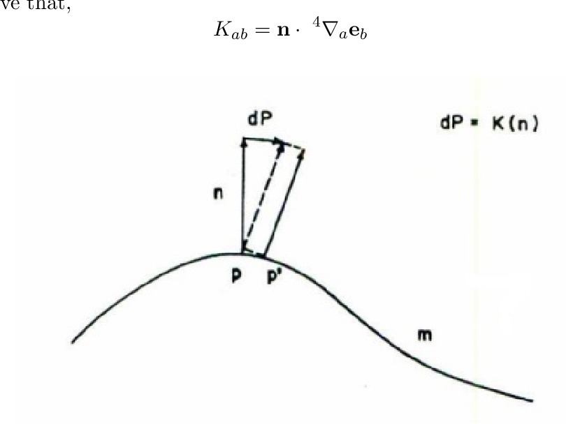
2. Formal Definition and Properties

With this intuition, we can now state the formal definition. The extrinsic curvature tensor $K_{\mu \nu }$ is defined by taking the covariant derivative of the normal vector field $n_{\beta }$ along a direction tangent to the hypersurface, and then projecting the result back onto the hypersurface.

As defined in the text, the extrinsic curvature is:

Let's unpack this:

• ${\nabla }_{\alpha }{n}_{\beta }$ is the change in the normal vector $n_{\beta }$ as we move in the direction of $x^{\alpha }$.
• ${\gamma }_{\mu }^{\alpha }$ and ${\gamma }_{\nu }^{\beta }$ are the spatial projection operators we defined in the last lesson (${\gamma }_{\mu }^{\alpha }={\delta }_{\mu }^{\alpha }+n^{\alpha }{n}_{\mu }$). They ensure that we are only considering derivatives along directions within the slice and that the resulting tensor is purely spatial.
• The negative sign is a common convention in the field.

From this definition, two key properties are immediately apparent, as noted in the resource:

1. $K_{\mu \nu }$ is a spatial tensor: By construction, it is orthogonal to the normal vector, $n^{\mu }{K}_{\mu \nu }=0$. This means it "lives" on the spatial hypersurface ${\Sigma }_t$, so we can write it with spatial indices as $K_{ij}$.
2. $K_{\mu \nu }$ is symmetric: $K_{\mu \nu }=K_{\nu \mu }$. The proof of this relies on the torsion-free property of the Levi-Civita connection $\nabla$ and is a fundamental result known as the Weingarten property.

3. Equivalent Definitions: Uncovering the Dynamics

The definition above is geometrically insightful, but other equivalent forms reveal the physical and dynamical meaning of $K_{ij}$ more directly.

A. The Lie Derivative Form

A powerful way to think about $K_{ij}$ is in terms of the Lie derivative. It can be shown that the extrinsic curvature is proportional to the Lie derivative of the spatial metric ${\gamma }_{\mu \nu }$ with respect to the normal vector $n^{\mu }$:

This equation is profound. The Lie derivative ${\mathcal{L}}_n{\gamma }_{\mu \nu }$ measures how the spatial metric is distorted as it is "dragged" an infinitesimal distance along the normal vector's flow field. In the context of our foliation, this flow is essentially the evolution into the future. Therefore, $K_{ij}$ measures the rate of change of the spatial geometry itself as time progresses. This is why it is the "velocity" variable.

The proof involves expanding the Lie derivative and is an excellent exercise in the tensor calculus you've learned.

B. The "Dynamical" Form

The most important form for practical calculations and for the Hamiltonian formulation relates $K_{ij}$ to the coordinate time derivative of the spatial metric, ${\dot{\gamma }}_{ij}\equiv {\partial }_t{\gamma }_{ij}$. In the previous lesson, we introduced the result:

Here, $D_i$ is the 3D covariant derivative compatible with the spatial metric ${\gamma }_{ij}$. The terms involving the shift vector, $D_i{N}_j+D_j{N}_i$, represent the Lie derivative of the metric along the shift vector, ${\mathcal{L}}_{\vec{N}}{\gamma }_{ij}$. So this can also be written as:

This equation makes the role of $K_{ij}$ as the canonical momentum conjugate to ${\gamma }_{ij}$ explicit. It isolates the "true" time evolution of the metric (${\partial }_t{\gamma }_{ij}$) from changes due to coordinate dragging (${\mathcal{L}}_{\vec{N}}{\gamma }_{ij}$) and rescales it by the lapse $N$.

4. Connecting Curvatures: The Gauss-Codazzi Equations

We have now established that a spatial slice has both an intrinsic curvature (${}^{(3)}R$) and an extrinsic curvature ($K$). How do these relate to the full 4D curvature of spacetime (${}^{(4)}R$)? The answer lies in the Gauss-Codazzi equations, which are fundamental structural equations in the 3+1 formalism.

The Gauss equation is particularly illuminating. It states that the projection of the 4D Riemann tensor onto the spatial slice is the sum of the slice's intrinsic Riemann tensor and terms quadratic in the extrinsic curvature:

(Note: this is a slightly rearranged version of the equation in some texts.) This equation shows explicitly how the curvature experienced by observers living in the 4D spacetime (${}^{(4)}R$) is composed of the curvature intrinsic to their spatial slice (${}^{(3)}R$) plus a contribution from how that slice is bending in time ($K_{ij}$).

Taking the trace of this equation leads to a relation between the Ricci scalars, which is a generalization of Gauss's famous Theorema Egregium:

Here, $K={\gamma }^{ij}{K}_{ij}$ is the trace of the extrinsic curvature. These equations will be the starting point for deriving the constraint equations in our next lesson.

Conclusion

In this lesson, we have thoroughly investigated the extrinsic curvature tensor $K_{ij}$, the second fundamental quantity in the 3+1 decomposition of gravity.

Key Takeaways:

• Geometric Meaning: The extrinsic curvature $K_{ij}$ measures how a spatial hypersurface ${\Sigma }_t$ is bent or embedded within the 4D spacetime manifold.
• Formal Definition: It is defined as the projected covariant derivative of the normal vector, $K_{\mu \nu }=-{\gamma }_{\mu }^{\alpha }{\gamma }_{\nu }^{\beta }{\nabla }_{\alpha }{n}_{\beta }$.
• Dynamical Meaning: It is equivalent to the rate of change of the spatial metric along the normal direction, $K_{\mu \nu }=-\frac{1}{2}{\mathcal{L}}_n{\gamma }_{\mu \nu }$.
• Practical Formula: For computation, it is expressed in terms of the time derivative of the metric and derivatives of the shift vector: $K_{ij}=\frac{1}{2N}({\dot{\gamma }}_{ij}-D_i{N}_j-D_j{N}_i)$.
• Structural Role: The Gauss-Codazzi equations show that $K_{ij}$ provides the crucial link between the intrinsic curvature of the spatial slices and the full curvature of spacetime.

Preview of the Next Lesson:

We have now assembled all the necessary mathematical objects: the configuration variable ${\gamma }_{ij}$, its conjugate momentum $K_{ij}$, and the non-dynamical lapse $N$ and shift $N^i$. In our next lesson, "Derive the Hamiltonian and momentum constraint equations of General Relativity," we will put these pieces together. We will project the full Einstein Field Equations onto our spatial slice and along the normal direction, using the Gauss-Codazzi relations, to arrive at the fundamental evolution and constraint equations that govern the dynamics of spacetime in the ADM formalism.