Smooth Manifolds: Charts, Atlases, and the n-Sphere

1. The Intuitive Idea: Locally Euclidean Spaces

Before diving into formal definitions, let's build some intuition. The core idea of a manifold is that it's a space where every point has a neighborhood that is "topologically equivalent" to an open disk in Euclidean space. "Topologically equivalent" (the technical term is homeomorphic) means you can continuously deform one into the other without cutting or gluing.

The surface of the Earth is a classic example. Globally, it's a curved sphere, but any small region (like your city) can be mapped onto a flat piece of paper (a map) without gross distortion.

This "locally Euclidean" property is what will allow us to eventually do calculus on these more general spaces.

To formalize this, we start with the concept of a topological manifold. Please watch the first few minutes of the following lecture by Frederic Schuller, which introduces this idea.

Let's unpack the technical conditions mentioned in the video:

• Hausdorff: Any two distinct points can be separated by disjoint open sets. This is a "sanity check" condition that prevents pathological spaces where points are "indistinguishable." All familiar spaces like ${\mathbb{R}}^n$ are Hausdorff.
• Second-countable / Paracompact: These are related conditions that, roughly speaking, prevent the space from being "too big" or having "too many holes." They ensure we can use tools like integration and partitions of unity, which will be important later. The lecture notes from the University of Hamburg, "Differential Geometry," provide a concise definition of these prerequisites on pages 1-2 (Definition 1.2) if you'd like a text reference. You don't need to dwell on the deep topological implications now, but it's important to know they are part of the formal definition.

The most important part of the definition is the existence of a homeomorphism (a continuous map with a continuous inverse) from a neighborhood of any point in our space $M$ to an open set in ${\mathbb{R}}^D$. This is the mathematical embodiment of the "locally looks like ${\mathbb{R}}^D$" idea.

2. Making it Concrete: Charts, Atlases, and Transition Maps

The homeomorphisms that make a space a manifold are the tools we use to assign coordinates locally. We give them special names.

• A chart is a pair $(U,\varphi )$, where $U$ is an open subset of the manifold $M$, and $\varphi :U\to {\mathbb{R}}^n$ is a homeomorphism onto its image, $\varphi (U)$. The map $\varphi$ is our "coordinate map." For a point $p\in U$, the vector $\varphi (p)\in {\mathbb{R}}^n$ gives the coordinates of $p$ in that chart.
• An atlas is a collection of charts $\{(U_i,{\varphi }_i)\}$ such that the open sets $U_i$ cover the entire manifold, i.e., ${\bigcup }_i{U}_i=M$.

Think of the atlas on the Earth again. Each page is a chart, providing coordinates (latitude and longitude) for a region. The whole book is an atlas, and together, the maps cover the entire globe.

Now, a crucial question arises: What happens in the regions where two maps overlap? A city like London might appear on a map of the UK and also on a map of Europe. It will have different coordinates on each map. We need a way to relate these coordinate systems to ensure consistency.

This is done via a transition map. If two charts, $(U_i,{\varphi }_i)$ and $(U_j,{\varphi }_j)$, overlap on the manifold ($U_i\cap U_j\ne \varnothing$), we can construct a map that goes from the coordinates in one chart to the coordinates in the other. The map
${\varphi }_j\circ {\varphi }_i^{-1}:{\varphi }_i(U_i\cap U_j)\to {\varphi }_j(U_i\cap U_j)$
takes coordinates from chart $i$ and gives back the corresponding coordinates in chart $j$. Notice that this is a map from an open subset of ${\mathbb{R}}^n$ to another open subset of ${\mathbb{R}}^n$. This is a familiar object from multivariable calculus!

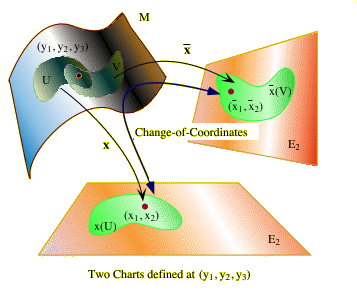
The properties of these transition maps are what determine the type of manifold we are dealing with. The following extensive video segment explains this framework in detail.

As the video notes, for a purely topological manifold, the transition maps are just continuous (C${}^0$), which is guaranteed by the definition. To do differential calculus, we need more structure.

3. Adding Smoothness

The learning outcome is to define a smooth manifold. We are now ready to do so. The "smooth" property is endowed upon the manifold by placing a stronger requirement on the atlas.

A smooth atlas is an atlas where all transition maps, ${\varphi }_j\circ {\varphi }_i^{-1}$, are not just continuous, but are smooth (infinitely differentiable, or $C^{\infty }$).

Why is this so important? It guarantees that the notion of "differentiability" is consistent across the manifold. If we have a function $f$ on the manifold and we find that its coordinate representation in chart $i$ is differentiable, the smoothness of the transition map ensures that its representation in chart $j$ will also be differentiable. This allows us to define what a smooth function on a manifold is, without ambiguity.

A smooth manifold is formally defined as a second-countable, Hausdorff topological space $M$ equipped with a maximal smooth atlas.

• The "maximal" part is a technical convenience. It means we consider the atlas to contain every possible chart that is smoothly compatible with the ones we started with. As explained in Lemma 1.10 of the "Differential Geometry" PDF (page 4), any smooth atlas uniquely determines a maximal one, so in practice, we only need to specify one valid smooth atlas to define the manifold's smooth structure.

4. Example: The n-Sphere $S^n$

Let's put this all together with a concrete example: the n-sphere, defined as the set of points in ${\mathbb{R}}^{n+1}$ at unit distance from the origin:
$S^n=\{x\in {\mathbb{R}}^{n+1}\mid \Vert x\Vert =1\}$
We can show this is a smooth manifold by constructing a smooth atlas for it. An atlas with just two charts is sufficient. These charts are constructed using stereographic projection.

1. Chart 1: Let $p_N=(0,\dots ,0,1)$ be the "North Pole." Our first open set is $U_N=S^n\setminus \{p_N\}$. The chart map ${\sigma }_N:U_N\to {\mathbb{R}}^n$ projects a point $x=(x_1,\dots ,x_{n+1})$ from the North Pole onto the equatorial hyperplane.
2. Chart 2: Let $p_S=(0,\dots ,0,-1)$ be the "South Pole." Our second open set is $U_S=S^n\setminus \{p_S\}$. The chart map ${\sigma }_S:U_S\to {\mathbb{R}}^n$ projects from the South Pole.

The following resource provides the explicit formulas for these maps and calculates the transition function to prove it is smooth.

The map $x\mapsto x/\Vert x{\Vert }^2$ is called an inversion. Its components involve rational functions whose denominators are never zero on the domain of the transition map (${\mathbb{R}}^n\setminus \{0\}$). Therefore, it is infinitely differentiable, the atlas is smooth, and $S^n$ is a smooth manifold.

Summary and Next Steps

Let's recap the key ideas from our first lesson.

• A smooth manifold is a space that locally resembles Euclidean space ${\mathbb{R}}^n$. More formally, it is a second-countable, Hausdorff topological space.
• We use charts $(U,\varphi )$ to assign local coordinates to points on the manifold. A collection of charts that covers the whole space is an atlas.
• The "smoothness" of the manifold is encoded in the requirement that the transition maps between any two overlapping charts must be infinitely differentiable ($C^{\infty }$).
• A smooth manifold is rigorously defined as a topological space equipped with a maximal smooth atlas.
• We demonstrated that the n-sphere $S^n$ is a smooth manifold by constructing a smooth atlas for it using two stereographic projection charts.

You now have a foundational understanding of the "arena" in which general relativity is formulated. However, a stage is empty without actors. We need to be able to define physical quantities on the manifold, like velocities, forces, and fields.

In our next lesson, we will take the first step in this direction by constructing the tangent space at a point on a manifold. This will lead us to the concept of vector fields, which are the manifold's generalization of the vector functions you are familiar with from electromagnetism and fluid dynamics.