Penrose Diagram of Kerr Spacetime's Maximal Analytic Extension

1. Strategy: A Patchwork of Spacetime Regions

The Boyer-Lindquist coordinates $(t,r,\theta ,\varphi )$ are singular at the outer and inner horizons, $r=r_{+}$ and $r=r_{-}$, where $\Delta =r^2-2Mr+a^2=0$. Our goal is to find new coordinates that are smooth across these surfaces.

The strategy, as meticulously detailed in the provided notes by C. R. C., is to construct the maximal geometry as an infinite sequence of alternating "blocks." We'll define coordinate patches that are regular around the outer horizon, $D(r_{+})$, and patches regular around the inner horizon, $D(r_{-})$, and then see how they are "glued" together.

Let's begin by focusing on the region around the outer horizon, $r_{+}$. The process is analogous to the construction of Kruskal-Szekeres coordinates: we define new null coordinates that remain finite as one approaches the horizon.

The construction you just reviewed builds a chart that covers four distinct regions, which we label with standard conventions:

• Region I ($\bar{I}$ in the text): Our asymptotic universe, $r>r_{+}$.
• Region II ($\bar{I}\bar{I}$ in the text): The black hole interior, $r_{-}<r<r_{+}$.
• Region I' (${\bar{I}}^{\prime }$): Another asymptotic universe, connected to ours through a past horizon. This is a white hole region.
• Region II' ($\bar{I}{\bar{I}}^{\prime }$): The white hole interior.

The diagram in Figure 7 shows how these four regions meet at the "crossing sphere" where $U_{+}=V_{+}=0$, which corresponds to the outer horizon $r=r_{+}$. An observer starting in Region I can cross the future event horizon ($V_{+}>0,U_{+}=0$) and enter the black hole interior, Region II.

2. Crossing the Inner Horizon and Beyond

Once an observer is in Region II ($r_{-}<r<r_{+}$), they are inexorably drawn towards smaller values of $r$. They will soon encounter the inner horizon at $r=r_{-}$. The coordinates $(U_{+},V_{+})$ are singular here. To see what lies beyond, we need a new coordinate patch, $D(r_{-})$, built analogously to handle the $r=r_{-}$ surface.

This second extension reveals what happens after an observer crosses the inner horizon $r=r_{-}$. This surface is a Cauchy horizon. Crossing it leads into a new type of region:

• Region III: The region inside the inner horizon, $0<r<r_{-}$.

This process doesn't stop. The full maximal extension is constructed by gluing together an infinite number of these $D(r_{+})$ and $D(r_{-})$ blocks.

3. The Maximal Kerr Spacetime: An Infinite Tower

The complete structure is an infinite ladder of universes. From our universe (Region I), one falls into a black hole interior (Region II). From there, one falls through a Cauchy horizon into Region III. This region acts as a gateway. From Region III, one could fall into the singularity, or one could pass through another Cauchy horizon into a new black hole interior (II'), from which one could emerge through a new event horizon into an entirely new universe (I'). This pattern continues indefinitely.

The schematic in Figure 9 is correct, but a more detailed and conventional diagram will help us analyze the physics. The following image provides a beautiful, clear rendering of the Penrose diagram for the maximal analytic extension of the Kerr spacetime.

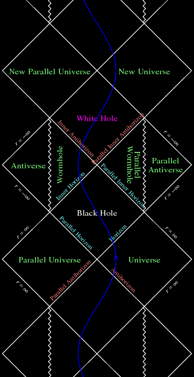
The presentation slides below also provide a clean, standard version of this diagram and summarize the construction.

4. Interpreting the Kerr Penrose Diagram

Let's dissect the features of this remarkable structure, using the diagrams from the resources as our guide.

• The Singularity ($r=0$): Unlike the spacelike singularity in Schwarzschild (a horizontal line at the top of the diagram that spans all of space), the Kerr singularity is represented by a vertical line. This indicates it is timelike. An observer falling into the black hole (i.e., on a timelike worldline) is not guaranteed to hit it. An observer who crosses the event horizon ($r_{+}$) and the Cauchy horizon ($r_{-}$) can maneuver to avoid the singularity and pass through the ring into a region with $r<0$, effectively entering a new universe.

• The Cauchy Horizon ($r=r_{-}$): The inner horizon is a Cauchy horizon. This is a null surface beyond which the future is no longer uniquely determined by initial data on a surface like ${\mathcal{I}}^{-}$. Predictability breaks down. Moreover, this horizon is known to be violently unstable to perturbations. Any infalling radiation gets infinitely blueshifted from the perspective of an observer crossing the horizon, creating a singularity there. This suggests the interior structure of a real, physical Kerr black hole might not match this idealized mathematical solution.

• Closed Timelike Curves (CTCs): Region III, between the Cauchy horizon and the singularity, is causally pathological. It contains closed timelike curves. This means an observer in this region could, in principle, travel along a trajectory that brings them back to their own past. This region is a "time machine." The existence of CTCs is another reason why the physical relevance of this interior solution is highly debated.

Conclusion

By analytically extending the Kerr metric, we have uncovered a breathtakingly complex spacetime structure. The Penrose diagram serves as our map to this bizarre landscape, guiding us through an infinite tower of universes connected by rotating black holes and white holes.

Key Takeaways:

• The maximal analytic extension of Kerr spacetime is constructed by patching together coordinate systems that are regular at the outer ($r_{+}$) and inner ($r_{-}$) horizons.
• This extension reveals an infinite repeating structure of asymptotically flat "universes" (Region I), connected through black hole interiors (Region II) and regions containing the singularity (Region III).
• Unlike the spacelike singularity in Schwarzschild, the Kerr ring singularity is timelike and can be avoided by an observer who falls into the black hole.
• The inner horizon $r=r_{-}$ is a Cauchy horizon, a surface beyond which predictability breaks down. This horizon is believed to be unstable in any realistic physical scenario.
• The region inside the Cauchy horizon contains closed timelike curves, violating causality and acting as a "time machine."

The pathological features of the Kerr interior—the Cauchy horizon instability and CTCs—have led to intense study and suggest that while the exterior Kerr metric is an excellent model for astrophysical black holes, the maximal extension may be a mathematical idealization rather than a physical reality.

Preview of Next Lesson:

This lesson completes our initial exploration of the causal structure of black holes. We will now move on to a more formal description of their properties. In the next lesson, we will define surface gravity ($\kappa$) for a stationary black hole. This quantity, which can be thought of as the force required at infinity to hold a particle stationary at the horizon, will turn out to be a cornerstone of the laws of black hole mechanics and their profound connection to thermodynamics.