Quantum Fields Near Black Hole Horizons

1. The Arena: Near-Horizon Geometry of a Black Hole

To study quantum effects near an event horizon, we must first understand the geometry of that region. We'll work with the simplest case: the static, uncharged Schwarzschild black hole. You'll recall the metric is:
$d{s}^2=-\left(1-\frac{2GM}{r}\right)d{t}^2+{\left(1-\frac{2GM}{r}\right)}^{-1}d{r}^2+r^{2}d{\Omega }^2$
The event horizon is located at the Schwarzschild radius, $r_s=2GM$. Notice that the coefficient of $d{t}^2$ goes to zero and the coefficient of $d{r}^2$ diverges as $r\to r_s$. This coordinate singularity makes calculations difficult.

To remedy this, we introduce the tortoise coordinate, $r_{\ast }$. This new radial coordinate is designed to "stretch" the horizon out to infinity, making the spacetime geometry near it more manageable.

As the reading explains, the tortoise coordinate is defined by $d{r}_{\ast }=\frac{dr}{1-2GM/r}$, which integrates to:
$r_{\ast }=r+2GM\ln \left(\frac{r}{2GM}-1\right)$
In terms of $(t,r_{\ast })$, the radial-temporal part of the Schwarzschild metric becomes:
$d{s}^2=\left(1-\frac{2GM}{r}\right)(-d{t}^2+d{r}_{\ast }^2)$
This form is very revealing. It is conformally flat—it looks just like the flat 2D Minkowski metric $-d{t}^2+d{r}_{\ast }^2$ multiplied by a position-dependent conformal factor.

Now, consider the region very close to the horizon, where $r\approx 2GM$. Here, we can approximate the conformal factor:
$1-\frac{2GM}{r}=\frac{r-2GM}{r}\approx \frac{r-2GM}{2GM}$
From the definition of $r_{\ast }$, we have $r_{\ast }\approx 2GM\ln (r-2GM)$, so $r-2GM\propto e^{r_{\ast }/(2GM)}$. Defining a coordinate $\xi =2GM\cdot e^{r_{\ast }/(2GM)}$ and a rescaled time, you can show that the near-horizon metric takes the form:
$d{s}^2\approx \frac{{\xi }^2}{(4GM{)}^2}(-d{t}^2)+d{\xi }^2$
This is precisely the Rindler metric we studied in the last lesson! The surface gravity $\kappa =\frac{1}{4GM}$ plays the role of the acceleration $a$. This confirms our intuition from the Equivalence Principle: the geometry for a stationary observer near the horizon is locally Rindler spacetime.

2. Quantization in a Curved Background

Having established the geometry, we now need to set up the rules for quantum field theory.

The key steps to formulate QFT on a curved background are:

1. Start with the covariant action for a scalar field $\varphi$:
   $S[\varphi ]=\int d^{4}x\sqrt{-g}\left(-\frac{1}{2}{g}^{\mu \nu }{\nabla }_{\mu }\varphi {\nabla }_{\nu }\varphi -\frac{1}{2}{m}^2{\varphi }^2\right)$
2. Derive the equation of motion, which is the Klein-Gordon equation in curved spacetime:
   ${\square }_g\varphi -m^2\varphi =0,\text{where}{\square }_g=\frac{1}{\sqrt{-g}}{\partial }_{\mu }(\sqrt{-g}{g}^{\mu \nu }{\partial }_{\nu })$
3. Expand the field operator in a basis of mode solutions $u_i(x)$ to this equation:
   $\hat{\varphi }(x)={\sum }_i\left({\hat{a}}_i{u}_i(x)+{\hat{a}}_i^{†}{u}_i^{\ast }(x)\right)$

The central challenge, as discussed in the reading, is the vacuum ambiguity. In a general curved spacetime, there is no global timelike Killing vector, and thus no unique way to separate modes into positive and negative frequencies. This means there is no unique, universally agreed-upon vacuum state.

3. Defining "In" and "Out" States for a Black Hole

For a Schwarzschild black hole that forms from collapse, the spacetime is asymptotically flat in the distant past and the distant future. This allows us to define two distinct, physically meaningful vacuum states.

To visualize this, we use a Kruskal-Szekeres diagram, which represents the maximal analytic extension of the Schwarzschild spacetime.

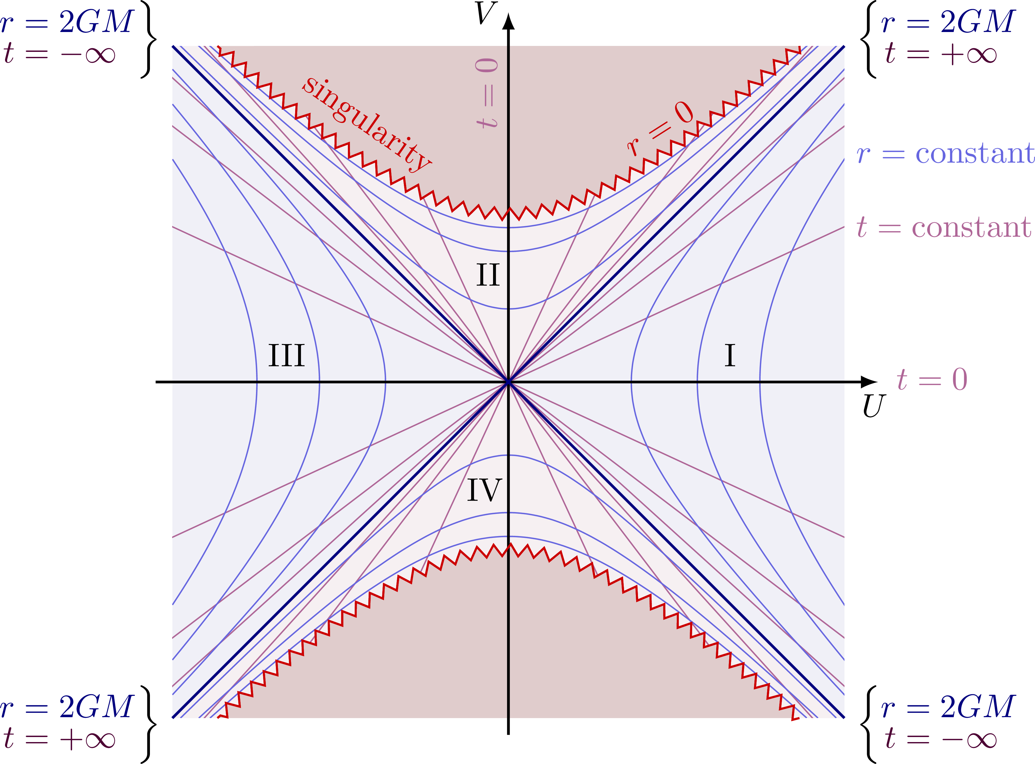
We can now define our quantum states:

• The "In" State: A hypothetical observer at past null infinity, ${\mathcal{J}}^{-}$, before the black hole has a strong influence, would see a standard vacuum. We can define a set of positive-frequency modes $\{f_i\}$ with respect to the standard time coordinate there. The vacuum state defined by these modes, where ${\hat{a}}_i|0_{in}⟩=0$ for all $i$, is called the Hartle-Hawking vacuum. It represents a state with no incoming particles from the distant past.

• The "Out" State: A different observer at future null infinity, ${\mathcal{J}}^{+}$, measures outgoing particles. They will define their own set of positive-frequency modes, $\{p_i\}$, corresponding to particles that escape the black hole. However, not all modes from the past reach ${\mathcal{J}}^{+}$. Some fall into the black hole. Therefore, a complete basis for modes in the future requires two sets:

  1. Modes $\{p_i\}$ that propagate to ${\mathcal{J}}^{+}$.
  2. Modes $\{q_i\}$ that propagate into the future horizon and hit the singularity.

The formalism is laid out nicely in the following resource.

To summarize the structure:

1. The field operator $\hat{\varphi }$ can be expanded in the "in" basis $\{f_i\}$ defined on ${\mathcal{J}}^{-}$.
   $\hat{\varphi }={\sum }_i(f_i{\hat{a}}_i+f_i^{\ast }{\hat{a}}_i^{†})$
2. The same operator can be expanded in the "out" basis $\{p_i,q_i\}$ defined on ${\mathcal{J}}^{+}$ and the future horizon.
   $\hat{\varphi }={\sum }_i(p_i{\hat{b}}_i+p_i^{\ast }{\hat{b}}_i^{†})+{\sum }_i(q_i{\hat{c}}_i+q_i^{\ast }{\hat{c}}_i^{†})$
3. Since $\{f_i\}$ is a complete basis, the outgoing modes $\{p_i\}$ can be written as a linear combination of the ingoing modes:
   $p_i={\sum }_j({\alpha }_{ij}{f}_j+{\beta }_{ij}{f}_j^{\ast })$
   This is our familiar Bogoliubov transformation. The physical question of Hawking radiation boils down to this: if the universe starts in the "in" vacuum $|0_{in}⟩$, what is the number of outgoing particles detected by an observer at ${\mathcal{J}}^{+}$? The answer is given by the expectation value of the "out" number operator:
   $⟨N_i⟩=⟨0_{in}|{\hat{b}}_i^{†}{\hat{b}}_i|0_{in}⟩={\sum }_j|{\beta }_{ij}{|}^2$
   If the coefficients ${\beta }_{ij}$ are non-zero, it means the observer at infinity will detect particles, even though none were sent in. The black hole's gravitational field has "created" them.

4. The Entangled Vacuum

What is the physical nature of this Hartle-Hawking vacuum state near the horizon? The simple picture of particle-antiparticle pairs being created, with one falling in and one escaping, is a useful heuristic. The deeper reality lies in the structure of quantum entanglement.

As Susskind explains, for an infalling observer to pass through the horizon smoothly (as predicted by the Equivalence Principle), the quantum state of the vacuum must be highly entangled between modes just inside and just outside the horizon. This is the true nature of the Hartle-Hawking vacuum. The "particles" of Hawking radiation are, in a sense, a consequence of the observer at infinity only having access to one part of this entangled system (the "out" modes), while the other part (the "in-falling" modes) is traced over.

5. A More Rigorous Formulation (Optional)

Given your interest in the mathematical foundations, it's worth noting that this entire structure can be put on a completely rigorous axiomatic footing, generalizing the Wightman axioms of QFT to curved spacetime.

This axiomatic approach provides a powerful confirmation of our physical picture: the geometry of a causal horizon, when combined with the principles of quantum field theory, inevitably leads to thermal phenomena.

Conclusion

In this lesson, we have constructed the complete theoretical framework for describing quantum fields near a black hole's event horizon. You have accomplished the essential steps needed to tackle the derivation of Hawking radiation.

Key Takeaways:

• By using tortoise coordinates, the near-horizon geometry of a Schwarzschild black hole can be shown to be locally equivalent to Rindler spacetime, providing a concrete link to the Unruh effect.
• Quantizing a field in this background requires defining separate sets of modes for ingoing particles (at ${\mathcal{J}}^{-}$) and outgoing particles (at ${\mathcal{J}}^{+}$ and the horizon).
• The vacuum state for an infalling observer, the Hartle-Hawking vacuum ($|0_{in}⟩$), is not seen as empty by a distant observer. The relationship between the "in" and "out" bases is described by a Bogoliubov transformation.
• The particle content of the outgoing radiation is determined by the Bogoliubov coefficient $\beta$, which measures the mixing of positive and negative frequency modes.
• Conceptually, the Hartle-Hawking vacuum is a state that is highly entangled across the event horizon.

Preview of the Next Lesson:

We have set the stage perfectly. All the conceptual and formal machinery is in place. In our next lesson, we will get our hands dirty and perform the calculation. We will explicitly compute the Bogoliubov coefficients ${\beta }_{ij}$ by tracing the "in" modes from ${\mathcal{J}}^{-}$ past the collapsing star, near the horizon, and out to ${\mathcal{J}}^{+}$. This will allow us to derive the Hawking temperature of a Schwarzschild black hole.