Introduction
In our last lesson, we focused on using data validation to control the information going into your cells, ensuring consistency and accuracy. This is a key step in building a reliable dataset. Now, we'll take the next logical step in organizing your work: connecting data across different sheets within the same spreadsheet.
As a data researcher, you'll often find it's cleaner to keep raw data, summaries, and different categories of information on separate sheets. This lesson will teach you how to "pull" data from one sheet to another dynamically. This means if the source data changes, your summary sheet updates automatically, saving you from error-prone copy-pasting and keeping your reports live. By the end of this lesson, you will be able to link cells and ranges across multiple sheets, a foundational skill for creating dashboards and consolidated reports.
The Anatomy of a Cross-Sheet Reference
When you reference a cell on the same sheet, you just use its A1 notation, like A1 or B2. To reference a cell on a different sheet, you simply add two components to the beginning of that reference: the name of the sheet and an exclamation mark.
The syntax is: SheetName!CellReference
For example, to get the value from cell C5 on a sheet named "SalesData", the reference would be: =SalesData!C5
One crucial rule: if your sheet name contains spaces or special characters, you must wrap the name in single quotes.
For example, for a sheet named "Q1 Sales", the reference would be: ='Q1 Sales'!C5
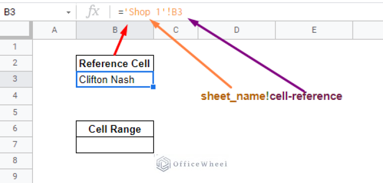
To solidify your understanding of this structure, please review the following short guide.
How To Reference Another Sheet in 2026 (+ Examples)
This article from Sheets for Marketers provides a clear, step-by-step breakdown of the syntax for creating cross-sheet references.
Read from the beginning of the article down to the end of Step 5. This will walk you through the logic and formatting of the formula.
The Easiest Way to Link Sheets
While typing the formula manually is good for understanding, the fastest and most common way to create a reference is by simply clicking. Google Sheets will build the formula for you automatically.
Here's the process:
- Select the cell where you want the data to appear.
- Type the equals sign (
=). - Click on the tab of the sheet you want to pull data from.
- Click on the specific cell you want to reference.
- Press Enter.
The video below demonstrates this process perfectly. It's the method you'll likely use most often in your day-to-day work.
Google Sheets | How to Reference Cells in Other Sheets
This video from Prolific Oaktree shows the intuitive point-and-click method for creating a link between sheets.
Watch from this section. The instructor first explains the concept and then demonstrates how to create a reference by navigating between sheets after typing the equals sign. Notice how Google Sheets automatically adds the single quotes when the sheet name has a space.
Once the formula is entered, the cell in your active sheet will mirror the value from the source cell.
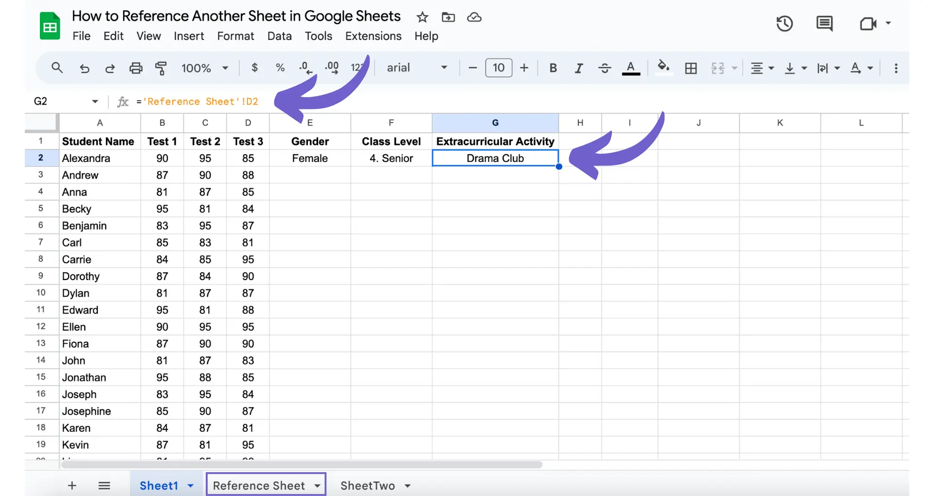
Working with Ranges and Functions
The power of cross-sheet referencing truly shines when you start working with entire ranges of data and embedding them within other functions.
Referencing a Range
You can pull an entire column or block of data, not just a single cell. The syntax is the same, but you use a range reference like A1:A100. For example: ='Q1 Sales'!B2:B50 will pull the data from all those cells.
Combining with Functions
This is where the magic happens for data analysis. You can perform calculations on data that lives on another sheet. For instance, you could sum up a whole column of sales figures from a "Raw Data" sheet without ever bringing the individual numbers into your "Summary" sheet.
Let's see how this works in practice, including a clever trick for copying these formulas.
Google Sheets | How to Reference Cells in Other Sheets
Continuing with the same video, these clips demonstrate how to apply these references to multiple cells and use them within a SUM function.
First, watch the segment on dragging formulas. This shows how you can create one reference and then drag the fill handle to quickly pull in data from adjacent cells in the source sheet. Next, watch the section on using the SUM function. This is a critical technique. It shows how you can build a formula that directly calculates values from another sheet, creating a truly dynamic summary.
Hands-On Exercise: Building a Sales Summary
Let's put this into practice.
- Open a new, blank Google Sheet.
- Rename the default sheet to "Sales Data". Click the small arrow on the "Sheet1" tab at the bottom and select "Rename".
- In the "Sales Data" sheet, set up a simple table:
- In cell A1:
Product - In cell B1:
Sales Q1 - In cells A2:A5:
Widget A,Widget B,Widget C,Widget D - In cells B2:B5:
150,220,95,180
- In cell A1:
- Now, add a new sheet by clicking the
+icon in the bottom-left corner. Rename this new sheet "Summary". - In the "Summary" sheet, we'll pull in the total sales.
- In cell A1, type:
Total Q1 Sales - In cell B1, type the following formula:
=SUM('Sales Data'!B2:B5)
- In cell A1, type:
- Press Enter. The cell should now display
645.
Go back to the "Sales Data" sheet and change one of the sales numbers. For example, change cell B3 to 100. Now, switch back to the "Summary" sheet. You'll see the total has automatically updated to 650. You've created a live, dynamic link!
A Look Ahead: Linking Separate Spreadsheets
So far, we've linked sheets within the same spreadsheet file. But what if a client sends you their sales data in a completely separate file? For a freelance data researcher, this is a common scenario.
Google Sheets has a powerful function called IMPORTRANGE designed for this exact purpose. It allows you to pull data from a different Google Sheets file altogether, just by using its URL.
We won't go into a full exercise on this today, but it's important for you to know it exists. The video below gives a clear demonstration of how it works.
How to Link Data Between Sheets and Spreadsheets in Google Sheets
This video from Teacher's Tech provides an excellent tutorial on the IMPORTRANGE function.
Watch the section from the beginning of the IMPORTRANGE explanation. Pay attention to the two main arguments the function needs: the spreadsheet's URL and a text string specifying the sheet and range (e.g., "Sales!B5:E5"). Note that you have to grant access the first time you link to a new spreadsheet.
Conclusion
You've now learned how to connect the dots within your spreadsheets, creating organized and dynamic reports. This skill is crucial for separating raw data from your analysis, which is a best practice in data research.
Here are the key takeaways from today's lesson:
- The fundamental syntax for referencing another sheet is
SheetName!CellReference. - If a sheet name contains spaces, you must enclose it in single quotes, like
'My Data'!A1. - The easiest way to create a reference is to type
=and then use your mouse to click on the desired sheet and cell. - You can reference entire ranges and use these cross-sheet references inside functions like
SUMto perform live calculations. - For linking to completely different spreadsheet files, the
IMPORTRANGEfunction is the tool for the job.
This lesson concludes our module on advanced spreadsheet techniques. You now have a strong foundation for collecting, cleaning, and structuring data within Google Sheets. In our next module, we will shift our focus to the "research" part of your goal: learning how to effectively find and gather information from the web. We'll begin with the most important tool in any researcher's arsenal: advanced Google search operators.