Turing Machine Space Complexity

1. From Time to Space: A New Measure of Complexity

Just as time complexity measures the number of steps a Turing Machine takes, space complexity measures the number of tape cells it uses. A key difference, however, is that a tape cell can be read from and written to many times, whereas a time step is consumed only once. This suggests that space might be a more powerful, reusable resource than time.

Let's begin by watching a video that introduces the formal definition of space complexity for both deterministic and nondeterministic Turing Machines.

Let's summarize and formalize the key points from the video.

Formal Definition

Let $M$ be a deterministic Turing machine (DTM) that is a decider (i.e., it halts on all inputs). The space complexity of $M$ is the function $s:\mathbb{N}\to \mathbb{N}$, where $s(n)$ is the maximum number of distinct tape cells that $M$ scans on any input of length $n$.

• If the space complexity of $M$ is $s(n)$, we say that $M$ runs in SPACE($s(n)$).
• For a nondeterministic Turing Machine (NTM), the space complexity is the maximum number of tape cells it uses on any single branch of its computation.

Notice the parallel to time complexity. We always consider the worst-case input of a given length $n$. For NTMs, we consider the maximum resource usage on any one path to an answer, not the sum across all branches.

For a more detailed textual definition and an example, you can review the following document.

An important subtlety, mentioned in the Washington.edu lecture notes (LINK), is that for many problems, the smallest meaningful space complexity is $O(\log n)$. This is because $\log n$ space is often required just to maintain a pointer or counter for the input tape, which has length $n$.

2. Multi-Tape vs. Single-Tape Machines

In our study of time complexity, we learned that converting a multi-tape TM to a single-tape TM incurs a quadratic time overhead. Does a similar penalty apply to space? Let's find out.

As the video explains, the simulation is much more efficient in terms of space. To simulate $k$ tapes on a single tape, we can simply lay out the contents of the $k$ tapes one after another. If the original machine used $s_1(n),s_2(n),\dots ,s_k(n)$ space on its tapes, the single-tape machine will use ${\sum }_{i=1}^k{s}_i(n)$ space (plus some small overhead for markers). This is a linear overhead, not quadratic. This robustness across machine models is a key property of space complexity.

3. The Relationship Between Time and Space

We've now defined two fundamental computational resources. A natural question arises: how are they related? Knowing the time complexity of an algorithm must tell us something about its space complexity, and vice versa.

The following video segment explains the two fundamental relationships between time and space.

Let's break down these two critical results. Let $f(n)$ be a function where $f(n)\ge n$.

1. TIME(f(n)) ⊆ SPACE(f(n))
   This relationship is straightforward. In one time step, a Turing Machine can move its head at most one cell. Therefore, a TM that runs for $f(n)$ steps cannot possibly visit more than $f(n)$ distinct tape cells. Its time bound is an upper bound on its space usage.

2. SPACE(f(n)) ⊆ TIME(2^(O(f(n))))
   This is a more profound result. It shows that any problem solvable with a certain amount of space can be solved in a corresponding amount of exponential time. Why?
   The proof relies on the number of possible configurations of the TM. A configuration is a snapshot of the machine at one instant, defined by:

   • The current state of the finite control.
   • The contents of the tape being used.
   • The position of the tape head.

   If a TM uses $f(n)$ space, let's count the number of distinct configurations.

   • Number of states: a constant, $|Q|$.
   • Number of head positions: $f(n)$.
   • Number of possible tape contents: If the tape alphabet is $\Gamma$, there are $|\Gamma {|}^{f(n)}$ ways to write symbols on $f(n)$ cells.

   The total number of configurations is the product: $|Q|\times f(n)\times |\Gamma {|}^{f(n)}$. This entire expression is exponential in $f(n)$, which we write as $2^{O(f(n))}$.
   Since our TMs are deciders, they must halt. If a TM runs for more steps than the total number of unique configurations, it must have repeated a configuration. If it repeats a configuration, it will loop forever. Therefore, the running time must be bounded by the number of configurations. This gives us the exponential time bound.

4. Space Complexity Classes

Just as we grouped problems into time complexity classes like P and NP, we can do the same for space.

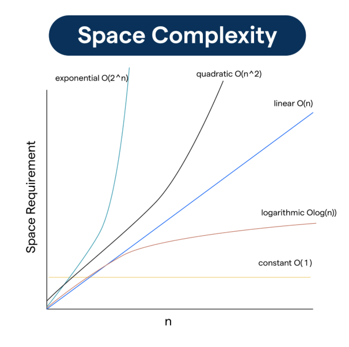
The formal definitions for space complexity classes mirror those for time:

• SPACE(f(n)) is the class of languages that are decidable by a deterministic Turing machine using $O(f(n))$ space.
• NSPACE(f(n)) is the class of languages that are decidable by a nondeterministic Turing machine using $O(f(n))$ space.

This framework allows us to define major classes based on polynomial space bounds, which you will explore in the next lesson.

Conclusion

In this lesson, we have formally defined space complexity and established its core properties. This provides us with a new dimension for analyzing the difficulty of computational problems.

Key Takeaways:

• Space complexity of a Turing Machine is the maximum number of tape cells it scans on any input of a given length $n$.
• For an NTM, space is measured as the maximum used on any single computational branch.
• Unlike time, converting a multi-tape TM to a single-tape TM incurs only a linear space overhead.
• Time and space are fundamentally related:
  • Any problem solvable in $f(n)$ time is solvable in $f(n)$ space: TIME(f(n)) ⊆ SPACE(f(n)).
  • Any problem solvable in $f(n)$ space is solvable in exponential time with respect to that space: SPACE(f(n)) ⊆ TIME(2^(O(f(n)))).

Preview of the Next Lesson:
Now that we have formally defined space complexity, we are ready to explore one of the most important complexity classes built upon this concept: PSPACE. This is the class of all problems decidable by a deterministic Turing Machine using a polynomial amount of space. In the next lesson, we will define PSPACE, investigate its properties, and explore its relationship to the familiar time-based classes P and NP.