Understanding NP-Completeness: NP-Hard and NP-Complete

1. A Tool for Comparing Hardness: Polynomial-Time Reduction

To say a problem is "the hardest," we first need a formal way to compare the difficulty of two different problems. The tool for this is called a polynomial-time reduction.

The intuition is this: if we can transform any instance of Problem A into an equivalent instance of Problem B, quickly (in polynomial time), then Problem B must be at least as hard as Problem A. If we had an efficient "black box" solver for B, we could use it to efficiently solve A.

We denote this relationship as $A{\le }_{p}B$, which reads "A is polynomially reducible to B."

To see a formal definition and explanation of this fundamental concept, please watch the following video.

To cement this idea with mathematical precision, let's look at the formal definition from a set of university lecture notes.

A key takeaway is that if $L_1{\le }_p{L}_2$ and we have a polynomial-time algorithm for $L_2$, we can construct a polynomial-time algorithm for $L_1$. Conversely, if we prove that $L_1$ cannot be solved in polynomial time, then $L_2$ cannot be solved in polynomial time either. The reduction transfers hardness from one problem to another.

2. Defining the Hardest Problems: NP-Hard and NP-Complete

With the tool of polynomial-time reduction, we can now formally define the classes of the "hardest" problems.

NP-Hard

A problem (or language) $L$ is NP-hard if every problem $L^{\prime }$ in NP is polynomially reducible to it.

This means that an NP-hard problem is at least as hard as every single problem in NP. If you could solve an NP-hard problem efficiently, you could solve everything in NP efficiently.

Importantly, an NP-hard problem does not have to be in NP itself. For example, the Halting Problem, which we know is undecidable, is also NP-hard. It's far harder than any problem in NP.

NP-Complete

A problem $L$ is NP-complete if it meets two conditions:

1. $L$ is NP-hard.
2. $L$ is in NP.

NP-complete problems are therefore the "hardest problems within NP." They are the problems that are both difficult enough to capture the complexity of the entire class NP, while still being verifiable in polynomial time.

Let's watch a short video that crisply states these two definitions.

For a textual reference, these articles provide excellent, complementary definitions.

The relationship between these classes is best understood visually.

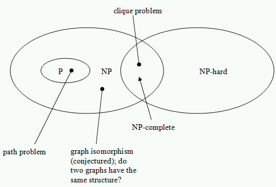
3. The Grand Implication: NP-Completeness and P vs. NP

The discovery of NP-completeness was revolutionary because it provided a direct line of attack on the P vs. NP problem. It connects the fate of thousands of disparate problems to the fate of a single one.

The central theorem of NP-completeness states:
If any NP-complete problem can be solved in polynomial time, then P = NP.

Why is this true? The logic follows directly from our definitions.

Let's summarize the argument from the video:

1. Assume you find a polynomial-time algorithm for some NP-complete problem, let's call it $L_{NPC}$.
2. Now, take any problem $L$ from the class NP.
3. By the definition of NP-completeness, we know there is a polynomial-time reduction from $L$ to $L_{NPC}$. Let's say this reduction takes $O(n^k)$ time. The size of the output might be $O(n^k)$.
4. You can then use your algorithm for $L_{NPC}$ to solve this new instance. Let's say your algorithm runs in $O(m^j)$ time, where $m$ is the input size. For our new instance, this is $O((n^k{)}^j)=O(n^{kj})$ time.
5. The total time to solve $L$ is the time for the reduction plus the time for solving: $O(n^k)+O(n^{kj})$, which is still a polynomial in $n$.
6. Since $L$ was an arbitrary problem in NP, this means every problem in NP can be solved in polynomial time. Therefore, P = NP.

This is an incredibly powerful result. It means that to prove P = NP, one only needs to find a polynomial-time algorithm for a single NP-complete problem, such as the Traveling Salesperson Problem, 3-Coloring, or the Knapsack problem.

Of course, this raises a crucial question: how do we know any NP-complete problems even exist? This was answered by the Cook-Levin Theorem (1971), which proved that the Boolean Satisfiability Problem (SAT) is NP-complete. This was the first domino. Once one NP-complete problem was found, others could be identified by creating polynomial-time reductions from SAT.

Conclusion

Today, we've moved from the abstract P vs. NP question to a concrete framework for classifying hard problems. This has given us a new, more focused way to approach the problem.

Key Takeaways:

• We compare the hardness of problems using polynomial-time reductions ($A{\le }_{p}B$), which formally means "B is at least as hard as A."
• A problem is NP-hard if every problem in NP can be polynomially reduced to it.
• A problem is NP-complete if it is both NP-hard and is itself in the class NP. These are the hardest problems within NP.
• The theory of NP-completeness provides a powerful link: if a polynomial-time algorithm is found for just one NP-complete problem, then all problems in NP can be solved in polynomial time, and P = NP.
• The Cook-Levin Theorem established the existence of the first NP-complete problem (SAT), paving the way for identifying thousands more.

Preview of the Next Lesson:
Our entire discussion hinges on the existence of that first NP-complete problem. In the next lesson, we will dive into the Cook-Levin Theorem. While we won't go through the entire proof in all its detail, we will understand its high-level structure and appreciate why the Boolean Satisfiability Problem (SAT) was the natural candidate. We will then see how, with SAT as our anchor, we can use reductions to prove that other famous problems are also NP-complete.