Designing Turing Machines for Formal Languages

Hello! Welcome back to your journey into the theory of computation.

In our last session, we learned how to formally trace the execution of a Turing Machine using Instantaneous Descriptions (IDs). This gave us a powerful tool to analyze a TM's step-by-step behavior. Today, we shift our focus from analysis to synthesis. Our goal is to design Turing Machines to accept formal languages, with a special focus on the classic example of $L = {a^{n} b^{n} c^{n} ∣ n \geq 0}$ .

This language is a significant milestone in our course. You'll recall that Pushdown Automata could handle ${a^{n} b^{n}}$ by using a stack to match a's and b's. However, matching three different symbols in equal number is beyond the capability of a PDA. This is where the true power of the Turing Machine—its ability to move back and forth and repeatedly modify its tape—becomes essential. Designing a TM for this language is a fundamental exercise that showcases what makes TMs the most powerful model of computation we will study.

1. From Tracing to Designing: The Core Strategy

Just as you would outline an algorithm before writing code, designing a TM starts with a high-level strategy. For languages that involve "counting" or matching symbols, a common and effective technique is to systematically "mark off" or "cross out" symbols in a specific order.

For $L = {a^{n} b^{n} c^{n}}$ , the strategy is a natural extension of the one we saw for ${a^{n} b^{n}}$ :

Find the leftmost, unmarked a and replace it with a marker (e.g., X).
Scan right, past any other a's and markers, until you find the leftmost, unmarked b. Replace it with a different marker (e.g., Y).
Continue scanning right, past any b's and markers, to find the leftmost, unmarked c. Replace it with a third marker (e.g., Z).
Once one of each symbol is marked, rewind the tape head all the way back to the left, positioning it just after the first block of markers.
Repeat this entire process.
If, at any point, the machine expects to find a symbol (e.g., a b after marking an a) and cannot, the string is malformed, and the machine should reject.
After all a's have been turned into X's, the machine performs one final sweep to ensure no unmarked b's or c's remain. If only markers are left, the machine accepts.

This "zigzag" process of scanning back and forth is a classic TM design pattern.

2. Developing the Strategy from Scratch

It's one thing to read a strategy, but another to see how it's developed. The following video provides an excellent "live solve" of this problem, showing the thought process behind creating the TM.

Turing Machine Example: a^n b^n c^n

Watch this video from Easy Theory to see how the 'zigzag' strategy is developed and translated into a state machine. The presenter works through the logic from first principles, which is very helpful for building intuition.

Watch the entire video (about 14 minutes). Pay close attention to: How the problem is broken down into a sequence of marking and scanning actions. The logic for handling the end of the process: verifying that everything has been marked correctly. How the machine handles the empty string (the case where n=0). The reasoning for why incorrect inputs (e.g., aabcc) would cause the machine to get 'stuck' and reject.

3. Formalizing the Design: States and Transitions

Now that you have the intuitive strategy, let's formalize it. Each logical step of our algorithm will correspond to one or more states in the TM's finite control. The states act as the machine's memory of what it's currently trying to do.

Here's a breakdown of the states and their purposes, based on a common design pattern.

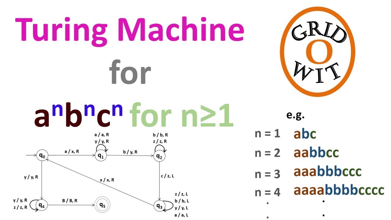
Turing Machine for a^n b^n c^n — A common state diagram for a TM accepting $L = \{a^n b^n c^n \mid n \ge 1\}$. This diagram uses X, Y, and Z as markers.

Let's walk through the logic of a machine like this:

q₀ (Start State): The initial state. Its job is to find the first a.
- If it sees an a, it writes an X, moves right, and transitions to q₁ to begin the search for a b.
- If it sees a Y right away, it means all a's have been processed. It transitions to q₃ to start the final verification.
- If the input is the empty string ( $n = 0$ ), it might see a blank. We'll add a path directly to an accept state for this case.
q₁ (Searching for b): This state's purpose is to find the corresponding b.
- It skips over any a's and Y's by reading them, writing them back unchanged, and moving right.
- When it finds the first b, it writes a Y, moves right, and transitions to q₂.
q₂ (Searching for c): This state is analogous to q₁; its job is to find the corresponding c.
- It skips over any b's and Z's.
- When it finds the first c, it writes a Z, moves left, and transitions to q₃ to begin rewinding.
q₃ (Rewinding): The purpose of this state is to return the tape head to the beginning of the next cycle.
- It moves left over all a's, b's, Y's, and Z's.
- When it finds the X that marks the start of the current scanned section, it moves one position to the right and transitions back to q₀ to repeat the cycle.
q₄ (Final Verification): This state is entered from q₀ when no more a's are found.
- It scans right over all the Y's and Z's.
- If it successfully scans past all the markers and finds a blank symbol (⊔), it means the string was valid. It moves to the accept state, q_{accept}.
- If it finds any stray b's or c's during this scan, the string is invalid, and the machine rejects (by having no defined transition).

To see another detailed construction of the state diagram and transitions, the following resource is helpful.

Turing Machines as Language Acceptors

This webpage from Old Dominion University provides another excellent walkthrough. It explicitly shows how the design for recognizing 0^n1^n2^n (equivalent to our a^nb^nc^n) is an extension of the design for 0^n1^n, which you saw in the last lesson.

Read the section '3.1 0^n1^n2^n'. Pay attention to the 6-step algorithm described, which mirrors the logic we just discussed. This reinforces the core design pattern.

4. A Concrete Trace

Let's tie this back to our previous lesson on tracing. Consider the input string abc and a TM designed for $n \geq 1$ .

Initial ID: q₀abc
Step 1: In q₀, read a, write X, move to q₁, move R.
q₀abc ⊢ Xq₁bc
Step 2: In q₁, read b, write Y, move to q₂, move R.
Xq₁bc ⊢ XYq₂c
Step 3: In q₂, read c, write Z, move to q₃, move L.
XYq₂c ⊢ Xq₃YZ
Step 4: In q₃, read Y, keep Y, stay in q₃, move L.
Xq₃YZ ⊢ q₃XYZ
Step 5: In q₃, read X, keep X, move to q₀, move R.
q₃XYZ ⊢ Xq₀YZ
Step 6: In q₀, read Y. This indicates no more a's are left. Move to q₄ to verify.
Xq₀YZ ⊢ XYq₄Z
Step 7: In q₄, read Z, keep Z, stay in q₄, move R.
XYq₄Z ⊢ XYZq₄⊔
Step 8: In q₄, read ⊔ (blank). All symbols were correctly paired. Move to the accept state.
XYZq₄⊔ ⊢ XYZ⊔q_{accept}⊔

The machine halts and accepts. If the input had been ab, the machine would have gotten stuck in state q₂ looking for a c, and would therefore reject.

Turing Machine Execution Trace and State Diagram for String Acceptance — This image visualizes a trace, connecting the tape's evolution (left) to the path taken through the state diagram (right). It helps solidify the link between the abstract design and the concrete computation.

Test your understanding!

The TM design we've discussed is for the language $L = {a^{n} b^{n} c^{n} ∣ n \geq 0}$ or $n \geq 1$ . The primary difference is how the empty string is handled.

Suppose you have a TM that correctly accepts $L = {a^{n} b^{n} c^{n} ∣ n \geq 0}$ . What single transition could you remove or change to make it accept for $n \geq 1$ instead?

Show answer

To change the language from $n \geq 0$ to $n \geq 1$ , you need to make the machine reject the empty string.

In a TM designed for $n \geq 0$ , the start state q₀ will typically have a transition for the blank symbol ⊔ that leads directly to the accept state. For example: δ(q₀, ⊔) = (q_{accept}, ⊔, R).

To modify the machine to accept for $n \geq 1$ , you would remove this transition. Without this rule, if the machine starts with a blank tape (the empty string), it will be in state q₀ reading ⊔, and since no transition is defined, it will halt and reject. All other non-empty strings will be processed as before.

Conclusion

Today, you've moved from an analyst to a designer of Turing Machines. You learned the fundamental "marking and scanning" strategy used to solve a whole class of problems that were previously unsolvable with simpler automata.

Key Takeaways:

Design starts with a high-level algorithm: Before defining states, map out the logical steps the machine will take.
States represent the machine's intent: Each state or group of states corresponds to a phase of the algorithm (e.g., "find a b", "rewind the tape").
The zigzag pattern is powerful: Scanning back and forth on the tape allows a TM to compare and count symbols across different parts of the input string.
$L = {a^{n} b^{n} c^{n}}$ is the canonical example of a language that is decidable by a TM but is not context-free, clearly demonstrating the superior power of the TM model.

Preview of the Next Lesson:
We've now seen how TMs can be used as language acceptors. In the next lesson, we will explore their other primary role: as function computers. We will design TMs that don't just give a yes/no answer but transform their input tape to produce an output, such as performing arithmetic operations like addition or copying strings.

Recommended resources

1. From Tracing to Designing: The Core Strategy

2. Developing the Strategy from Scratch

3. Formalizing the Design: States and Transitions

4. A Concrete Trace

Conclusion