Nondeterministic Turing Machines: Definition and Tracing

1. What is a Nondeterministic Turing Machine?

In a Deterministic Turing Machine (DTM), for any given state and tape symbol, there is exactly one possible next move. A Nondeterministic Turing Machine (NTM) relaxes this constraint, allowing for multiple possible moves at each step.

To get a clear initial picture of this difference, let's watch a short video.

Formal Definition of an NTM

As the video highlighted, the core difference lies in the transition function. Formally, a Nondeterministic Turing Machine is a 7-tuple $N=(Q,\Sigma ,\Gamma ,\delta ,q_0,q_{acc},q_{rej})$, where all components are the same as in a DTM, except for $\delta$.

The transition function for a DTM is:
$\delta :Q\times \Gamma \to Q\times \Gamma \times \{L,R\}$

In contrast, the transition function for an NTM is:
$\delta :(Q\setminus \{q_{acc},q_{rej}\})\times \Gamma \to \mathcal{P}(Q\times \Gamma \times \{L,R\})$

Let's break this down:

• $(Q\setminus \{q_{acc},q_{rej}\})\times \Gamma$: The input to the function is still the current non-halting state and the symbol under the tape head.
• $\mathcal{P}(...)$: This is the crucial part. $\mathcal{P}$ denotes the power set. This means the function's output is not a single triple, but a set of triples. This set can contain zero, one, or multiple possible transitions.

This formal definition captures the "choice" an NTM has. If $\delta (q,a)$ returns a set of three transitions, the machine can choose any one of them to follow.

For a more rigorous look at this definition, you can refer to the following text.

2. Tracing NTM Computation

Since an NTM can have multiple possible moves at each step, its computation is no longer a linear sequence of configurations. Instead, it's a computation tree, where the root is the starting configuration and the children of any node are all the configurations that can be reached in one step.

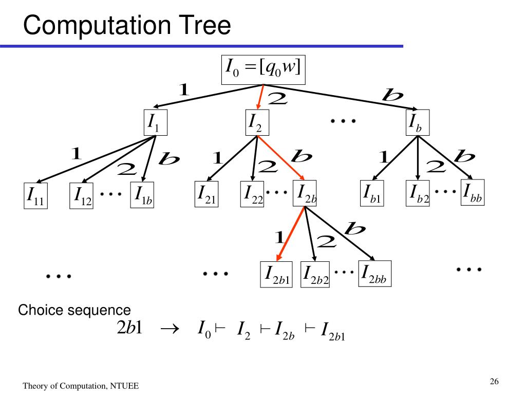
A visual representation of an NTM's computation. The root I₀ is the initial configuration. Each path from the root represents one possible sequence of choices the NTM can make.

Configurations and the "Yields" Relation

As a quick refresher, a configuration (or instantaneous description) is a snapshot of the TM's state, tape content, and head position, often written as uqv.

• q is the current state.
• u is the portion of the tape to the left of the head.
• v is the portion of the tape starting from the head position to the right.

The moves in the computation tree are formally described by the yields relation, denoted by ⊢. We write $C_1⊢C_2$ if configuration $C_2$ can be reached from $C_1$ in a single step according to one of the choices in the NTM's transition function.

Acceptance and Rejection in NTMs

The existence of multiple computation paths changes how we define acceptance. The rule is simple and analogous to that of NFAs:

• Accept: An NTM accepts an input string w if at least one branch of its computation tree leads to the accept state, $q_{acc}$.
• Reject: The NTM rejects w if all branches of the computation halt, and none of them reach the accept state.
• Loop: The NTM loops on w if there is no accepting branch and at least one branch continues forever.

Notice the asymmetry: a single accepting path is enough for the entire machine to accept, even if other paths reject or loop.

The following video segment explains this tree-based computation and the outcomes very clearly.

3. A Worked Example: L = {ww | w ∈ {a, b}*}

Let's see how nondeterminism can be a powerful design tool. Consider the language L consisting of all strings that are a word w repeated, like abab or bbaabbaa.

Designing a DTM for this is tricky. You'd have to shuttle back and forth, marking symbols to check for equality. An NTM, however, can solve this much more elegantly by "guessing."

Here's the high-level strategy for an NTM:

1. Guess: Nondeterministically move a second tape head (or a marker on a single tape) to the right, "guessing" where the midpoint of the input string is. For each possible midpoint, a new branch of computation is created.
2. Verify: Once a midpoint is chosen, deterministically compare the substring before the midpoint with the substring after it.
3. Accept/Reject: If the two substrings match perfectly, that computation branch accepts. If they don't match, that branch rejects.

If the input string is indeed in the form ww, then one of the "guesses" for the midpoint will be correct, and that corresponding computation branch will lead to acceptance. Therefore, the NTM as a whole accepts the string.

The following resource provides a sketch and a computation tree for this exact problem.

Test your understanding!

Consider the partial NTM computation tree shown in the image below for the input string abb. The notation on the edges is (read)/(write, move, new_state).

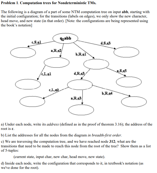
1. What is the full configuration of the node at address 2? (Assume the tape starts with the input and is otherwise blank.)
2. Follow the path from the root (address ε) to the node at address 21. What is the final configuration of this node?
3. If q3 were the accept state, would the NTM accept the input abb based on the partial tree shown? Why or why not?

Show answer

1. The node at address 2 is reached from the root q0abb by the transition a / (X, R, q2). The head reads a, writes X, and moves Right. The configuration is Xq2bb.

2. Let's trace the path to 21:

   • Root (ε): q0abb
   • Move 2: Apply a / (X, R, q2). Configuration becomes Xq2bb.
   • Move 1: From state q2 reading b, apply b / (b, R, q3). The head reads b, writes b (no change), and moves Right. The final configuration is Xbq3b.

3. Yes, the NTM would accept. The definition of acceptance only requires that one computational path reaches an accept state. Since the path to node 21 ends in state q3, this branch accepts, and therefore the entire machine accepts the input abb, regardless of what happens on other branches.

Conclusion

In this lesson, we formally introduced Nondeterministic Turing Machines. We saw that their power comes from the ability to explore multiple computational paths simultaneously, represented as a computation tree.

Key Takeaways:

• Formal Definition: An NTM's transition function $\delta$ maps a state-symbol pair to a power set of possible moves, $\mathcal{P}(Q\times \Gamma \times \{L,R\})$.
• Computation as a Tree: An NTM's execution on an input w generates a tree of configurations, where each branch is a possible sequence of choices.
• Acceptance Condition: An NTM accepts if any branch of its computation tree reaches an accepting state.
• Nondeterminism as a Tool: Nondeterminism allows us to design machines that "guess" a solution (e.g., the midpoint of a string) and then deterministically "verify" it. This can simplify the design process for certain languages significantly.

Preview of the Next Lesson:
We've defined NTMs and seen their utility. A critical question remains: are they more powerful than DTMs? Can they recognize languages that DTMs cannot? Following the pattern we saw with finite automata, the answer is no. In our next lesson, we will prove that NTMs and DTMs are equivalent in computational power. The proof involves a clever simulation where a DTM systematically explores the NTM's entire computation tree. Given your background in algorithms, you might appreciate that the simulation strategy is analogous to a breadth-first search.